| P. E. Lestrel, present address: 7327 De Celis Place, Van Nuys, CA 91406–2853, USA P. E. Lestrel, corresponding author. e-mail: plestrel@earthlink.net Published online 16 April 2004 in J-STAGE (www.jstage.jst.go.jp) DOI: 10.1537/ase.00069 |
“The study of form may be descriptive merely, or it may become analytical. We begin by describing the shape of an object in simple words of common speech: we end by defining it in the precise language of mathematics; and the one method tends to follow the other in strict scientific order and historical continuity,” quoted from D’Arcy Thompson (1915), Morphology and Mathematics.
It has long been recognized that the human cranial base (CB) acts as the major supporting structure for the brain and plays a pivotal position in the growth and development of the craniofacial complex (Bjork, 1955). There has also been the implicit assumption over the last half century that CB structures are relatively stable over both ontogenetic and phylogenetic time, although there is a paucity of evidence supporting this. While differences between males and females (sexual dimorphism) for many morphological structures (stature, weight, etc.) have been widely recognized, there is still little evidence available with respect to such changes in the craniofacial complex. Documented changes in the craniofacial structures tend to be primarily concerned with size, with little emphasis on shape. In the CB, evaluations of size and shape become quite complex, even when confined to two-dimensions, and the collection of such measurements is by no means a trivial endeavor. The introduction of this paper consists of two parts. The first part is an extended discussion of a number of theoretical issues that arise when measurement of form is considered. This is followed by the second part, which is a somewhat intuitive background for understanding Fourier descriptors, the Fourier transform, the short time Fourier transform and finally, wavelets. We felt that the rather extensive background discussion was justified for a better understanding and appreciation of wavelet theory.
What exactly do we mean by size and shape? How are these concepts related to form? Notions of size, shape, and form and their inter-relationships have been historically controversial. A cursory look at Webster’s Unabridged Dictionary (1983) reveals that form is defined as: “the shape or outline of anything; figure; image; structure, excluding color, texture and density.” Upon looking up shape one finds matters becoming more confused and tautological, with shape defined as: “... outline or external surface” or “the form characteristic of a particular person or thing”. According to these definitions, ‘shape’ and ‘form’ can be considered as interchangeable, to be viewed as essentially identical. Clearly, if this confusion between shape and form is to be alleviated, these concepts require re-definition, and this issue will be addressed in this paper. Moreover, besides problems of definition, there is the more challenging concern of how to measure size and especially the shape of forms. The traditional view has tended to ignore problems of measurement, on the grounds that a readily available approach, universally used, seemingly yielded acceptable results. This conventional approach consists of linear distances, angles, and ratios.
Difficulties continue to be present in spite of over a hundred years of such easily gathered measures. For example, little effort has been made to separate the effects of size and shape within the conventional metrical approach (CMA). It has been simply presumed that linear measures represent size, and angles or ratios (proportions) define shape. This is accurate only in the simplest sense. For example, consider the commonly utilized cranial base angle (nasion-sella-basion or NSB). This angular measure of the CB has been and continues to be controversial (Lestrel et al., 1993). One reason for this has to do, in part, with attempts to measure complex biological forms with a method that is not particularly suitable for that purpose. That is, CMA was designed for the measurement of regularly-shaped, i.e., non-natural (artificial) structures. It was never intended for the measurement of irregular forms of the type encountered in the biological sciences.
Nevertheless, investigators continue to use such measures seemingly unaware of the serious limitations that the use of such measures entail. This is not to suggest that conventional metrical measures such as the NSB cannot provide rough estimates of the angulation of the CB. They, in fact, do provide such estimates. However, it remains unclear as to what these CB angulation estimates really mean, since such measurements fail to describe the actual CB morphology as well as any changes that are taking place in the CB over time.
Every angle is composed of two lines and three points. Thus, changes at one, two or all three of the points (landmarks) may be involved in the angulation of the NSB, but it is not possible to identify precisely where the CB changes are occurring without independent confirmation (Lestrel et al., 1993). Thus, relying solely on NSB, it is not possible to determine whether the increase in angulation is due to superior migration of nasion, inferior movement of sella or the superior placement of basion. The NSB angle only reflects, in some complex and uncertain way, the shifting (or migrating) of the three landmarks involved as a function of the forces of bone resorption and deposition (Enlow, 1975). Any changes in the actual CB structures remain unknown, and thus, not measurable simply using the NSB angle or other measures.
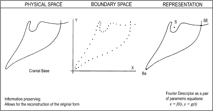
Another one of the deficiencies with CMA is illustrated in Figure 1. It is not possible to re-construct the original form from the measurements; that is, the information contained within the CB is not preserved with CMA. Thus, with CMA it is very difficult, if not impossible, to archive the measurements so that they can be used to re-create precisely the form at a later time. Such a ‘preservation’ or archiving capability requires other methods (see FDs below).
 View Details | Figure 1. The lateral view of the human cranial base with three homologous landmarks, being described with the conventional approach (CMA) composed of angles and distances. One of the limitations of CMA is that it is not possible to subsequently re-create the form from an archived data set consisting of traditionally derived measures. |
Other objections that have been raised against the use of the NSB angle are as follows: [1] nasion is not a cranial base landmark, it refers to the frontal bone, [2] sella has no structural reference, and most critical, [3] the NSB angle does not measure any actual aspect of the CB itself. Yet, it is this very question, of where the changes are occurring, that is one of the primary issues of interest in any analysis of the structures of the craniofacial complex. If CMA, composed of distances, angles and ratios, suffers from shortcomings, are there alternate methods that the researcher can draw on? The answer to this question can now be answered in the affirmative and will be addressed more fully later.
Finally, a separate issue is that biological organisms and their structures are, of course, three-dimensional (3-D) and this adds much more complexity in terms of the measurement of size and shape. In fact, one such study, of the rabbit orbit in 3-D, is instructive in terms of the difficulties that are encountered (Lestrel et al., 1997). The discussion that follows will, consequently, be limited to two-dimensional (2-D) data because of: [1] the relative ease in obtaining such data and [2] measurement problems arising at that level need to be resolved first.
Figure 2 is an attempt to illustrate this complexity in form. Note that six attributes are illustrated here. These six are: [1] scale (size), [2] outline (shape), [3] surface (texture), [4] interior (patterning), [5] color and [6] spatial orientation. Other attributes may need to be considered for a complete model of form. Of the above attributes, size and shape represent some of the more important ones from a quantitative perspective, and these will be emphasized here.
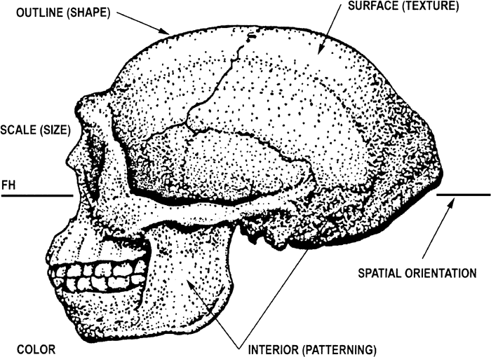 View Details | Figure 2. A number of attributes for determining form. Six such attributes are shown here: [1] scale (size), [2] outline (shape), [3] surface (texture), [4] interior (patterning), [5] color and [6] spatial orientation. Potentially, other attributes may be indicated but they are not shown here. |
Size is defined here as ‘scale’, and differences in size between organisms are often readily visually apparent. Measurement of size differences is not simple, because forms also differ in shape, which can act as a confounding factor. The use of CMA is particularly limited in this regard.
Shape is defined here as ‘outline’, and differences in shape between organisms are based on the boundary or contour in 2-D. The shapes of two organisms (limited to 2-D, but can be conceptually extended to 3-D), are identical, if and only if, their boundary outlines completely coincide everywhere (geometric congruence property). This requires that if one of the forms is smaller than the other, size scaling will also be required. Thus, the appropriate approach for examining differences in shape requires as a first step, the scaling of the forms so that they are equal in size. This can be accomplished for 2-D bounded forms by standardizing on area. For open curves, area is inadmissible so other standardizing approaches have been discussed, such as the perimeter (van Otterloo, 1991). For purposes here, the CB outline is scaled such that the bounded area becomes a constant value (see methods section). Finally, two other normalizations schemes have been proposed. One is based on Fourier energy considerations (Cesar and Costa, 1996) and the other the major axis (Cesar and Costa, 1998).
However, such a definition of shape, is of necessity, incomplete. It is incomplete in the sense that besides the overall boundary, many other aspects within a form also reflect the ‘shape’ attribute (e.g., consider the antero-superior border of the zygoma leading anteriorly to the supra-orbital ridge in Figure 2). As a consequence, two approaches to computational shape analysis have been recognized. These are: [1] boundary or contour-based and [2] region-based (Costa and Cesar, 2001). Nevertheless, the first shape definition, based on the boundary outline or contour, is intended as a starting point of reference here with respect to the Japanese CB and amply illustrates the complexities associated with measuring shape.
Textural considerations are largely involved with the two attributes: surface (texture) and interior (patterning). These two elements are intended to model: [1] the surface configuration of a form and [2] the interior structure (i.e., for example the cellular matrix of bone). The spatial orientation attribute refers to the orientation of a form in 2-D space (or 3-D space). A common orientation for superimposition is needed for the comparison of forms. While the color attribute is seemingly self-explanatory, problems of its measurement in terms of reflectance, luminescence, etc., remain to be fully explored in a biological context. Finally, it is again to be re-iterated that other attributes may need to be developed for a complete model of form.
But even this more complete model has to be joined with actual measurements before it can be reasonably applied to biological data such as the CB. This immediately raises three questions: [1] can measurements be objectively derived, [2] what measurements are appropriate and, [3] how many measurements are sufficient? The implications flowing from the first question have been scarcely addressed in spite of over a century of measurement. It is argued here that the very selection of measurements (e.g., consider a set of distances or angles) imparts subjectivity to the scientific endeavor. With respect to the appropriateness of a measure, it can be noted that the choice of a different set of measures taken on the same object, may have a decided effect on the final outcome. The third issue, sufficiency, has also received inadequate attention. How can we be sure that we have measured the total morphological form? It will be argued that sufficiency, in terms of the number of measurements used, remains an important and vexing problem which has been insufficiently recognized.
The complexities involved in the measurement of the other attributes such as the interior (patterning) and the surface (texture), as well as color, are certainly resolvable and necessary for a complete model of form. But they will be ignored for the time being. They represent work for the future. The research presented here will be confined largely to the size and shape properties of the Japanese CB.
Before we turn to the alternative methods proposed here as alternatives to CMA, we need to briefly consider the issue of homology. Considerable controversy has ensued as there are two rather diverse approaches (O’Higgins and Johnson, 1988; O’Higgins, 1997). These are traditional or biological homology and geometric homology. Traditionally, homology was never considered in terms of landmarks or points, but rather solely in terms of whole structures. Owen first formalized it in 1843 as the same organ in different animals (Owen, 1846). In contrast, the raw data for geometrical homology are landmarks, which are presumed, (if not always satisfying the criterion) to be in some sense ‘homologous’. Homology in geometric terms has been defined as a one-to-one mapping between corresponding points on different forms (Bookstein, 1991). Moreover, these points must also be biologically equivalent between organisms; otherwise, an analysis even if based on homologous points, can become biologically irrelevant. See Lestrel (1997a) for a more detailed discussion of some of the problems inherent with these definitions of homology. We will need to return to this seemingly inescapable issue of homology.
The last three decades have spawned a variety of new and mathematically more sophisticated methods to circumvent the limitations of CMA. These methods have been loosely grouped under the term morphometrics. Morphometrics can be viewed as a set of procedures, which facilitate the mapping of the visual information of form into a mathematical representation. Some of the morphometric methods used to analyze form can be placed into two broad categories, homologous-point and boundary-outline methods. Detailed discussions of these two contrasting views can be found in Read and Lestrel (1986) and Lestrel (1997b, 2000). However, these methods tend to be viewed as largely independent of each other because of the lack of a formal unifying model (Richtsmeier et al., 2002; Lestrel, in press). One boundary-outline technique of particular interest here, are Fourier descriptors (FDs). FDs have been successfully utilized for over three decades to quantify the outline of irregular contours.
Ever since the publication of J.B.S. Fourier’s seminal work on heat transfer in 1822, Fourier analysis has been of major importance, both from a mathematical viewpoint as well as an applied one (Grattan-Guiness, 1972; Herivel, 1975). Fourier analytic techniques continue to be extensively used in very diverse fields (Lestrel, 1997b). Fourier demonstrated that one can precisely reproduce almost any complicated curve or function by using sine and cosine terms of varying amplitudes and frequencies, which when summed (or more accurately, integrated) will converge onto any arbitrary curve (or function). This process, resulting in a precise emulation of the curve or function, using sinusoidal components, is called harmonic synthesis. This procedure of harmonic synthesis is particularly useful in that FDs can be used to re-create the outline of the form under consideration (information-preserving property), in contrast to landmark methods as previously discussed.
Fourier also showed that such a curve could be decomposed into separate elements (sines or cosines) as well. Today, the use of Fourier descriptors (FDs) refers to this decomposition of the function or curve into separate components or harmonics and is known as harmonic analysis, or more simply, Fourier analysis. These separate components (amplitudes, power, phase, etc.) can be considered as comprising the Fourier representation of the curve or signal. Another of these components is power, a measure of variance. Power is also called the power spectrum (all these terms will be defined in some detail later). Useful discussions can be found in Tolstov (1962), Kline (1972) and Davis (1986).
Fourier analysis can also be viewed as a transformation of data from one domain to another. In fields such as signal processing, this transformation is from the time domain into the frequency domain. In other fields such as pattern recognition and the biological and earth sciences, the transformation is generally from the spatial, rather than the time domain, into the frequency domain. For purposes here, the spatial domain refers to the data points that determine the boundary of the 2-D form, and the frequency domain is defined in terms of a new set of variables (coefficients) describing amplitude and phase relationships. This has also been termed a decomposition of the spatial configuration (boundary) into frequency components (amplitude and phase). Strictly speaking, all FDs are transforming methods, not just the somewhat misleadingly named Fourier transform (FT) to be discussed subsequently.
Three aspects of Fourier analysis deserve comment, these are: the period, the amplitude and the phase. Consider a simple sinusoidal function such as a sine wave, which repeats over an interval (along the x-axis). The period, L, refers to one complete cycle from 0 to 2π radians or 360 degrees. For the CB, our structure of interest here, this cycle, [0, 2π], is from the first point on the boundary to the last one. The frequency, on the other hand, is the reciprocal of this period or wavelength, f=1/L. This means that as the wavelength (period) gets smaller, the frequency will increase. The fundamental frequency is given by the first harmonic, which is, generally equal to the interval from [0, 2π] or [−π, π]. The next higher frequency is the second harmonic, which is one-half the wavelength of the fundamental frequency, and so on. The amplitude, in the Cartesian co-ordinate system, refers to the maximum height of the waveform from the x-axis (measured along the y-axis). As the frequency increases, the amplitude values tend to decrease. However, there may be exceptions to this rule. Phase refers to the displacement of the starting point of the waveform from the origin.
For example, the form of the sinusoidal curve, y=cos x, is identical to y=sin x, except that it is shifted in phase by 90 degrees or π/2 radians. These three properties: period, amplitude and phase provide a flexible system that can be used to fit many forms. The spatial form under consideration is made “periodic” in the sense that it is repeated over a set interval (the period), usually from 0 to 2π. That is, the last data point on the outline is followed by the first point, and the process is repeated (Lestrel, 1980, 1982). If any observed 2-D form can be described with a set of discrete points (x, y) on the boundary outline (generally equally spaced), then such a structure, represented as a tabulated function, can be fitted with a Fourier series.
If we define the period over a 2π interval, we can simplify the familiar discrete form of Fourier’s series in Cartesian form to: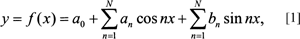
where a0 is a constant, an and bn are the Fourier coefficients, n is the harmonic number and x refers to the points sampled over the period along the x-axis, and N is the maximum harmonic number. The a0, an, and bn coefficients are computed from the following equations. While these are normally defined as integrals (the continuous case), the ones here refer to the discrete case, since actual data sets are usually in finite tabulated form (i.e., in a table). Sampling along an outline with even k divisions over the interval [−π, π], allows the constant, a0, and the coefficients, an and bn, to be computed
as:
and
where n is the harmonic number, The limits n=0 and n=k−1 above follow from the trapezoidal rule for computing areas (Harbaugh and Merriam, 1968; Lestrel, 1997b) and N is the maximum harmonic, subject to Nyquist or folding frequency requirements. For technical reasons having to do with signal processing and the Fourier transform (FT), the frequency spectrum (see below) is always symmetric (a mirror-image along the time axis) so that one part can be discarded or folded onto itself (Polikar, 1996).
The Nyquist frequency, is the maximum frequency, or highest harmonic, that can be detected from the sampled data. That is, sufficient samples (the data points on the biological form) must be taken to ensure that the peaks and valleys, the amplitudes in the frequency domain, will accurately depict the original form in the spatial domain. This is necessary to avoid noise or distortion, called ‘aliasing’, of the signal. Thus, the maximum number of harmonics, according to the Nyquist frequency, cannot exceed 1/2 the number of sampled data points (Newland, 1993).
The nth amplitude is defined as:
where An is the amplitude for the nth harmonic, an and bn are the respective Fourier coefficients, and n is the harmonic number. One procedure commonly utilized with FDs (and EFFs to be described subsequently), is to plot the amplitude (An) values as a function of the harmonic number, n. Since the amplitude is a frequency component, this plot is called a frequency spectrum. Moreover, from the amplitude one also can derive the variance or “power”, which is defined as the square of the amplitude and can also be plotted as a function of the harmonic number. This plot is called the power spectrum. This latter graph of power versus harmonic is particularly useful in that it is a description of the contribution that each harmonic makes toward the total form, in terms of the explained variance (Davis, 1986; Lestrel, 1997b).
The remaining property is phase. The phase angle for the nth harmonic is computed as: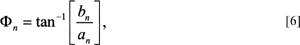
where the an and bn are again the coefficients for the nth harmonic.
Two other procedures need to be briefly mentioned. These are two normalizations termed positional orientation and size-standardization (Parnell and Lestrel, 1977; Lestrel, 1980). Positional-orientation refers to two aspects: [1] the orientation of the outline in space (the issue of phase) and [2] the placement of the center from which the vectors to the outline are constructed and measured (if in polar coordinates). The first aspect can be controlled with judicious positioning of the outline prior to digitization. The second aspect requires that a neutral center, the centroid, be computed. The centroid is the only center from which the position of the vectors remains invariant under rotation. The use of any other center results in increased variability in the Fourier coefficients (in a sense ‘noise’) due strictly to the position of the center, and not to the variability in the outline (Parnell and Lestrel, 1977; Full and Ehrlich, 1982).
The second normalization, size-standardization, is predicated on the grounds that shape, in contrast to size, contains considerable informational content of importance. This is not to imply that size is unimportant, but rather to stress again that measurement of shape can be unduly influenced by size or scale. If size differences are at all appreciable, subtle shape differences may be swamped and confounded. Three normalization approaches have been suggested: [1] based on the a0 or constant term, [2] based on the arc length or perimeter of the outline and [3] based on the bounded area. The first normalization refers to the constant of the Fourier series, a0, which is defined as the mean of the vectors from the centroid to the outline. Schwarcz and Shane (1969) were probably the earliest to apply this approach. Although this value is readily computed, and has been used as a scaling factor to control for size, it has the impediment that if the outline of interest departs significantly from a circle, the scaling factor will become increasingly inaccurate (Lestrel, 1980).
The second normalization, based on the perimeter, was discussed by van Otterloo (1991) as mentioned earlier, who applied it in a pattern recognition context. A possible drawback with this normalization is that it is dependent on the smoothness of the contour being sampled. That is, significant differences could arise with a scaling factor based on the perimeter. However, in the case of open rather than closed (bounded) curves, perimeter may be the only practical choice. The third approach, the one advocated here, is based on the area within the bounded outline (Lestrel, 1974).
FDs have been widely applied to structures ranging from sedimentology in geology (Thomas et al., 1995) to the biological sciences such as cell biology (Pesce Delfino et al., 1986; Strojny et al., 1987; Kieler et al., 1989; Diaz et al., 1990), botany (Kincaid and Schneider, 1983; White and Prentice, 1988; White et al., 1988) to anatomy (Lestrel, 1974, 1980, 1982, 1989b; Johnson, 1985, 1997; Inoue, 1990; Lestrel and Kerr, 1992, 1993) to mention only a few.
While many of the above methods have provided new data and useful information, FDs, and specifically elliptical Fourier functions (EFFs) to be discussed in the next section, are particularly well suited for characterizing the boundary outline of irregular morphologies, such as those encountered in the craniofacial complex. Specifically, FDs also remove one of the major deficiencies associated with the use of CMA; namely the inability of CMA to allow for the precise reconstruction of the shape of the form. Figure 3 illustrates the ability of EFFs to accurately re-construct the original CB, a particularly desirable goal in terms of archival of data.
 View Details | Figure 3. The lateral view of the human cranial base being fitted with a Fourier descriptor (FD); specifically, an elliptical Fourier function (EFF). Such an approach is information preserving, in that it allows for the subsequent re-creation of the form from the measurements. |
Elliptical Fourier functions (EFFs) are similar to other FDs in that they also transform the spatial domain into the frequency domain. EFFs, however, represent a specialized FD, one that it is generated from a parametric formulation. Parametric equations (Smail, 1953) are of the form: x=f(t), y=g(t), which allows for the separation of the boundary contour into separate x- and y-components. Computation is simpler and faster in CPU terms since the required computations do not use of integration. Integrals, Eqs. [2], [3] and [4], are required for evaluation of the Fourier coefficients with conventional FDs, Eq. [1], as well as the FT, Eqs. [10] and [11], which are more complex (see below). In contrast, EFF coefficients are computed using an algebraic approach.
Two of the constraints associated with conventional FDs are not applicable to EFFs namely: [1] an even number of intervals between points along the boundary outline and [2] the need to sample the boundary as a power of two (also required with FTs). As a consequence of the parametric formulation, multi-valued functions are now acceptable (Rohlf, 1990). These latter two aspects, acceptance of multi-valued functions and unequal spacing of points on the outline, confer particular advantages to the use of EFFs, by allowing for the numerical characterization of a much larger class of 2-D forms than previously possible (details can be found in Lestrel, 1997b, 2000).
The EFF equations were originally developed by Kuhl and Giardina (1982) and represent a parametric solution set up in the Cartesian coordinate system. The formulation consists of a pair of equations (x and y) derived as functions of a third variable (t). These parametric functions are set up as:
and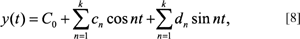
where n equals the harmonic number and k equals the maximum harmonic number. Solutions for the A0, C0, an, bn, cn and dn coefficients are required (for details of the procedures involved, see Kuhl and Giardina, 1982; Lestrel, 1989a, b, 1997b, 2000). Although this paper is largely limited to 2-D forms, it is of interest that if the boundary of a form can be modeled as a curve in 3-space (i.e., not as a volume), then the above equations can be extended without difficulty with the addition of a third parametric equation (Lestrel, 1997b). This parametric Fourier series in z(t) is:
The E0, en and fn coefficients being computed in an identical fashion to the 2-D case, Eqs. [7] and [8]. An application of such 3-D EFFs to characterize the boundary of the rabbit orbit can be found in Lestrel et al. (1997).
From these equations one can derive the usual values of amplitude and phase. However, a number of other estimates of certain geometric properties such as the area, perimeter, centroids and moments, have also been utilized (Kiryati and Maydan, 1989; van Otterloo, 1991). Since the above parametric formulations, either in 2-D or for a 3-D curve in space, produce ellipses, they provide a number of additional measures that are potentially useful as ‘similarity measures’ for clustering and discriminant procedures. These are ellipse area, perimeter, semi-major and semi-minor axes, as well as angulation of the major ellipse axes with the x-axis or with respect to other ellipses. All these estimates are separately computed for each harmonic.
Earlier, the issue of homology was raised and it is now examined within the framework of FDs. A limitation with conventional FDs, as well as FTs, has been the use of equally-spaced data. If homology of points is an issue (and with craniofacial data such as the CB data, it is), then it becomes apparent that it is not possible to incorporate homologous landmarks (irregularly located on the boundary) into a traditional FD, since equal divisions or intervals have to be maintained. Thus, one of the early criticisms of FDs was that the homology of points across forms was lost, and with it, the localization of boundary features.
With EFFs, this problem has been rectified. Homology is now maintained by a specific computational procedure. The first homologous predicted point is computed to be at the same location on the Fourier approximating (interpolating) function as the first observed point on the digitized form. The second and subsequent predicted points are computed so that they have the same arc length from the first computed point as their counterpart (observed) landmarks do from the first digitized point on the original, digitized form. This is equivalent to moving or translating the observed co-ordinates of the polygonal representation of the form, onto the EFF curve. The pseudo-homologous points are mapped from the digitized curve onto the EFF (Wolfe, 1997). These points have been termed pseudo-homologous; after the suggestions of Sneath and Sokal (1973). The mapping error must be kept very small since it is incumbent upon the investigator to keep the residual, the difference between the observed points and the predicted points derived from the EFF, as low as practically possible. Mean residual values based on all points should not rise above 0.1 percent, preferably less. That is, these values need to be well below the errors arising from such tasks as: [1] locating the points and [2] digitizing them.
These EFF computations maintain the homology of the points, and the entire form. While some loss is inevitable in regions of sharp curvature, this is usually minor and localized. Point homology can now be maintained, with the caveat that a sufficient number of homologous or pseudo-homologous points must be initially available. That is, the sampling along the boundary outline must always be composed of closely-spaced points to insure a close fit between the observed data and the predicted EFF. This technique can be considered as the first tentative step toward a model that now integrates the homologous point data with the boundary outline information (Lestrel, 1997b).
Numerous papers have appeared since the publication of the Kuhl and Giardina (1982) algorithm. These papers have ranged widely, from botanical applications (White and Prentice, 1988; White et al., 1988), and cell biology (Diaz et al., 1989, 1990, 1997; Nafe et al., 1992) to craniofacial structures such as the maxilla and mandible (Lestrel, 1987, 1997b; Ferrario et al., 1990, 1991; Lestrel et al., 1991). While the initial emphasis was directed toward pattern recognition (Lin and Hwang, 1987), publications, dealing with the shape of mosquito wings (Rohlf and Archie, 1984), and the outline of Mytilus edulis shells (Ferson et al., 1985) represent the initial extension of EFFs to a biological context. Rohlf and Archie (1984) compared the shape of mosquito wings using three FDs. These were conventional FDs, another FD approach (Zahn and Roskies, 1972), as well as EFFs. They found that EFFs produced the most satisfactory results in terms of discrimination.
A study of the primate cranial base in norma lateralis using EFFs normalized for size produced an almost perfect classification using discriminant functions (Lestrel et al., 1988). Of the four primate adult groups: [1] H. sapiens (n=31); [2] P. troglodytes (n=22); [3] G. gorilla (n=10); and [4] M. nemestrina (n=29), only one chimpanzee (P. troglodytes) was misclassified as a gorilla. A more recent primate study applied EFFs to characterize the shape of the cranial base in Macaca nemestrina (Lestrel et al., 1993). This study represented an extension of previous work using conventional FDs (Lestrel and Moore, 1978; Lestrel and Sirianni, 1982). Statistically significant changes were found for both sex and age. The age changes consisted of a gradual lengthening in the anteroposterior direction, with a simultaneous narrowing in the superoinferior direction. An elongation of the dorsal clivus, as well as an anterior migration of the hypophyseal fossa, was observed. These results have some bearing on the current study (see discussion). Work has also focused on precisely delineating the location of 2-D shape changes in the lateral view of the cranial base in shunt-treated hydrocephalics compared to normal age and sex matched controls (Lestrel et al., 1994; Lestrel and Huggare, 1997).
Thus, FDs, and EFFs in particular, can be considered as useful mathematical representations for numerically and visually documenting the global shape changes in complex 2-D morphologies encountered in the craniofacial complex. We now turn to another FD, this Fourier representation is called the Fourier transform or FT.
For a clearer understanding of wavelets, to be discussed subsequently, we need to briefly introduce the widely used Fourier transform (FT) and its newer ‘cousin’ the fast Fourier transform (FFT). In signal processing, transforms often provide information not easily obtainable from the original signal (the raw data).
This leads naturally to the question of what is a transform? A simple transform that everyone is generally familiar with is the procedure of taking logarithms. Here the transform is a procedure that simplifies the process of long division and multiplication. Figure 4 shows this procedure in a schematic fashion. On the left is the conventional approach; namely long division. While on the right is the transform approach which consists of looking up their log values, subtracting and then looking up the anti-log to obtain the answer. The FT is, of course, a bit more involved, but conceptually, the transform principle is the same.
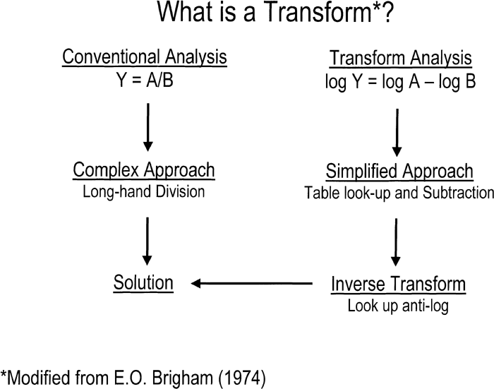 View Details | Figure 4. An example of a simple transform is the procedure of taking logarithms. By taking logs, subtracting, and then taking the anti-log, one can bypass long-division. |
For purposes here, since we are not involved with signal processing, which involves time as the major variable, we focus on ‘spatial data’, such as the CB. We can transform this ‘spatial data’ consisting of our measurements, from the spatial domain into the frequency domain. Once we are in the frequency domain, we will be dealing with sinusoidal elements (sines and cosines) at different frequencies. These sinusoidal components include amplitudes, power and phase. These parameters are again limited by the Nyquist frequency. We begin with our data (closely-spaced points along the CB boundary) and transform these into new frequency components such as amplitudes, etc. This new set of transformed variables can then be used for analysis and statistics. Some restrictions that must be met include: [1] the closely-located points along the CB boundary are usually sampled as a power of two (2n) such as 2, 4, 8, 16, 32, 64, 128, 256, 512 points, etc., and [2] the intervals between the points must be of equal length. Note: Homology of points is now lost. However, it should be noted that this power of two restriction is technically not a mathematically-derived restriction of the continuous FT, but rather a constraint of the fast Fourier transform (FFT), a widely-used algorithm for computing the FT (see below).
The continuous FT is a mapping from the time or spatial (boundary) domain into the frequency domain, in an exactly analogous way to FDs. The technique is composed of two parts (called a Fourier transform pair), which are the Fourier transform (FT) and the inverse Fourier transform (IFT). The first part, the FT, identifies the different frequency components (amplitudes) that characterize the function of interest, or f(t). These Fourier amplitude coefficients are complex, containing both real and imaginary sinusoidal components. This new function, X(f), is defined as:
where x(t) is the waveform to be decomposed into a sum of amplitude coefficients, X(f), as a function of the frequency. Thus, X(f) is the Fourier transform of x(t), e is the natural log base and i is imaginary, that is, equal to the square root of −1. The exponential function, e-i2πft, is called the kernel. The X(f) term on the left of the integral sign refers to the frequency domain. The x(t) term on the right of the integral sign refers to either the time or spatial domain. In the case of the CB it is the spatial domain and is defined as the sampling function along the boundary of the form. This function, x(t), is multiplied by a complex exponential term or kernel function, where f refers to the frequency along the x-axis, 2π refers to the period along the x-axis and t refers, by convention, to the ‘time’ axis. In this case this is the ‘spatial’ axis since we are dealing the boundary of forms. Note that the basis or kernel function, e-i2πft, above also equals cos 2πift+isin 2πift. This is an alternate expression (see Eqs. [12] and [13] below). Note that the i before the sin term indicates that the expression is complex.
It should be reiterated that the FDs (described earlier), as well as the FT here, represent a decomposition of the boundary contour (spatial domain) into different frequency sinusoids (frequency domain). The continuous FT represents a more general case, in that it can be used to analyze non-periodic phenomena in contrast to FDs, which require that the data be periodic. Non-periodic waveforms are those that do not repeat themselves over a set interval. Thus, the FD is simply a special case of the FT (Brigham, 1974; Challis and Kitney, 1991).
In more technical terms, consider a periodic function where each harmonic is separated by an amount Δf=1/L, where Δf is the change in frequency and L is the period. In brief, the FT is derived by taking the discrete Fourier series, converting it to complex-exponential form and then taking the limit so that the change in frequency, Δf, approaches zero as the period, L, approaches infinity (Brigham, 1974; Ramirez, 1985). A periodic or non-periodic waveform, given by f(t), can be transformed or decomposed from a function over time, f(t), (or space when dealing with forms) into a new function, containing sinusoidal frequency components or amplitudes.
Once the different frequency sinusoids are obtained, they can be combined to re-create the form used as a representation of the original function, f(t). For this purpose, a second equation is required, which is the IFT. This allows one to ‘transform back’ from the frequency domain function, X(f), and reconstruct the actual signal or spatial form, x(t). In other words, to recreate the waveform, x(t), from its Fourier transform:
The x(t) term now on the left of the integral sign refers to the time or spatial domain. The X(f) term on the right is the Fourier transform of x(t) and this function, X(f), is multiplied by a complex exponential term or kernel function.
Alternatively, Eqs. [10] and [11] can be re-expressed in terms of sine and cosines. Changing notation and simplifying by setting the period equal to a 2π interval, gives the discrete version of the Fourier transform (DFT) as:
and the inverse DFT as: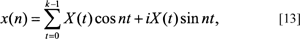
where the cosine term is the real nth component of the DFT and its inverse, and the sine term refers to the complex nth component and its inverse (modified from Ramirez, 1985). While these equations are not generally used for computational purposes in contrast to Eqs. [10] and [11], they do facilitate comparison with conventional FDs, and the EFFs described earlier.
The DFT represents computational advantages when used in conjunction with the FFT. Interestingly, it was the great German mathematician, Carl F. Gauss (1777–1855) who anticipated the FFT (Heideman et al., 1985). The FFT cuts down the computer time required to calculate the transform coefficients, which can become excessive as the number of harmonics increase (Hamming, 1973; Bracewell, 1989). Assuming that the number of multiplications involved (ignoring additions and general overhead) are proportional to CPU time, we can estimate the savings in CPU time. Using the conventional FT, CPU time increases by n2 where n is the number of points (samples), while with the FFT it only increases by n*log2 n. To make this more concrete, consider a contour with 512 points. Assuming an arbitrary time estimate, this would require 262,144 ms (or 4.37 min) with the FT. With the FFT, this reduces to 4,608 ms (or 4.61 sec), a 57-fold decrease or a 98.4% savings in CPU time! As a consequence, the FFT is now the preferred computational approach (Cooley and Tukey, 1965; Brigham, 1974; Ramirez, 1985; Newland, 1993).
One of the major drawbacks of FDs and FTs, is that while they provide frequency domain information (the frequency components such as amplitude and phase), they do not provide information with respect to where in the time domain these frequency components occur. In signal processing terms this means that while the spectral components in the signal are measurable, their location in time is not known. Equivalently, those components in the frequency domain also do not provide any information about their location in the spatial domain. Thus, while they are useful for capturing the global aspects of a form, the localization or identification of local aspects is not possible using Fourier coefficients or their amplitudes. This arises because these coefficients (or the amplitudes computed from them) are ‘smeared’, so to speak, over the whole form. That is, each coefficient or amplitude measures an aspect of the global or total form, but not any single localized feature.
In other words, FDs and FTs cannot deal adequately with signals or ‘spikes’ of short duration arising in the time domain. In the case of the CB or other morphologies, this would refer to the spatial domain where sharp curvature changes on the boundary could be viewed as singularities. In either case, such events of short duration, and of high frequency, cannot be easily isolated and numerically characterized by the Fourier coefficients or their amplitudes. It is in this sense that FDs and FTs are limited in their usefulness.
This is a consequence of the familiar Heisenberg uncertainty principle applied to signal processing. Heisenberg’s quantum mechanics principle states that you cannot simultaneously know the momentum and position of a moving particle. In signal processing this indeterminacy implies that you cannot identify the location of a signal simultaneously in the time (or space) and frequency domains. Namely, the more localized or precise the spike is in the time domain or the singularity in the spatial domain, the more uncertain is its location in the frequency domain. Conversely, the more precise the frequency information is, the more vague will be its location in time (or space). What is needed is a representation in which both the frequency components and their location in time (or space) are identifiable, and this is called a time-frequency representation. Thus, attempts at resolution of this localization deficiency of conventional FDs and especially FTs, led to the development of new approaches such as the short time Fourier transform (STFT) and eventually to wavelets (Lestrel, 2000).
Utilizing a totally different approach, EFFs allowed for a partial circumvention of this localization issue with the use of distances from the centroid to selected aspects on the boundary, thereby identifying localizing elements. However, a serious drawback is that this procedure was and remains subjective. Wavelets, on the other hand, provide a solution to the problem, although they do not completely solve it, in the sense that the uncertainly principle still applies (Hubbard, 1998). These two developments, the STFT and wavelets, have been largely confined to signal processing and pattern recognition engineering until recently (Nadler and Smith, 1993; Costa and Cesar, 2001). Both methods are briefly reviewed in the next two sections.
As mentioned above, the inability to identify position or localization of singularities has spawned new methods. It is of interest to note that the fact that the FT cannot be used to detect local events has been known for two centuries, and attempts to resolve this problem goes back to 1890 according to Costa and Cesar (2001, page 471). The wavelet transform (to be described in the next section) represents the most successful response to date to the inability of earlier Fourier methods to identify localized boundary phenomena. Prior to the wavelet transform however, an earlier approach was developed in an effort to deal with this lack of localization; in effect, a revision of the FT. This was the windowed or short time Fourier transform (STFT), which utilized a window concentrated around the origin. Recalling the FT as:
one can show that the window in this case can be viewed as covering the whole interval so that the presence of transients or spikes in the time domain (or singularities in the spatial domain) will affect the whole Fourier representation. Consequently, instead of these spikes or singularities being identified in the frequency domain, they become lost in the high frequency components. It was to rectify this problem that the STFT was developed.
Utilizing Eq. [10] we can add a window concentrated around the origin, which is shifted, starting at t=0 in the time domain (or s=0 in the spatial domain) along the time/boundary representation. This procedure was aimed at selecting only a small portion of the signal/boundary domain at a time. This prevents the influence of signal events outside this window from unduly affecting the whole Fourier representation (Costa and Cesar, 2001). Here the signal, x(t), is now multiplied by the window function, w(t), such that:
where b refers to the position of the window along the time/boundary, the w*(t−b) term defines the width of the window, with the * representing the complex conjugate (see Bolton, 1995, page 146 for an explanation of complex conjugates).
One can see that the STFT is simply the FT of the original signal multiplied by the window. Shown here is the continuous case of the STFT (there is also the discrete case—see Lestrel, 2000 for its formulation). This approach yields a time-frequency representation that allows for the identification of the location of the frequency components in the time/boundary domain. Specifically, using a narrow window allows for more precise frequency information about events in the time/boundary domain.
While the STFT (which predates wavelets) represents a substantial improvement over conventional FDs and FTs, it is based on a window function that is concentrated around the origin, one which has a constant width for all frequencies. Thus, the problem with the STFT approach is that by not being able to vary the window width, you are forced to choose a relatively wide window to attain good resolution of the frequency domain but at the expense of poor time resolution. Conversely, the choice of a narrow window to attain good resolution of the time domain (to identify peaks and other singularities) leads to poor resolution in the frequency domain (Polikar, 1996; Hubbard, 1998).
The wavelet transform represents the next natural step, allowing for a variable window shift in contrast to the constant window, characteristic of the STFT. This has been termed a multi-resolution approach, which is developed in more detail in the next section. Multi-resolution simultaneously allows for the recognition of high frequency elements, which are narrow in width as well as low frequency aspects, which are wide in width. This facilitates a much more precise localization in both the time/boundary and the frequency domains, providing wavelets with an advantage with respect to the STFT (Costa and Cesar, 2001).
The number of publications dealing with wavelets is literally in the thousands now, indicating the power and generality of the approach. Most of these papers, however, are still largely confined to the fields of mathematics, physics, pattern recognition, signal processing, machine vision and allied fields; although, applications are beginning to appear in other disciplines. In spite of the now undoubted usefulness of wavelets for characterizing the boundary outline of biological forms, there remains a paucity of such papers in the biological sciences. The following material is presented in a largely intuitive manner, with no attempt at a rigorous exposition (reference can also be made to the appendix, which outlines the specific wavelet used in the preparation of this paper). Readers who want to probe more deeply will need to consult the relevant literature. In keeping with earlier FD considerations, wavelets, as normally used in signal processing, also consists of a transformation of the time (or signal) domain into the frequency domain.
Since we are dealing here with the CB, the transformation is from the spatial domain into the frequency domain. In an exactly analogous manner to FDs, EFFs and the FT, where one derives coefficients based on the addition of sines and cosines to approximate the signal, or the boundary of a form, wavelets coefficients re-create the signal/boundary with the addition of wavelets of different sizes and at different positions (Hubbard, 1998).
In contrast to FDs however, the wavelets components are not sinusoidal. Thus, the first difference between FTs and wavelets rests on the lack of this periodicity. The second difference is that, FTs, besides being based on sinusoidal functions, also range over the period [−∞, ∞] for the continuous case. Wavelets, in contrast, are of limited duration and rapidly tend to zero at both ends of the interval (compact support, specifically for the discrete case). This results in a small ‘wave’, hence the name wavelets. Moreover, because of their finite duration they are narrowly focused in either time or space, and this allows for the identification of localized information of the frequency components in the time/boundary representation, a critical property missing with conventional FDs or FTs (Lestrel, 2000).
Specifically, wavelets are also a time-frequency representation, in that they use a small or narrow window to access high frequency components and a large or broad window to view low frequency components. It is the division of the signal/boundary domain into levels that is defined as a multi-resolution decomposition (Mallat, 1989). Wavelets have been characterized as a zoom lens, in that it allows one to focus on the broad landscape (low frequency components) as well as zoom in on the details in the scene (high frequency components). That is, the resolution of the wavelet transform varies with magnification, so to speak.
Thus, the wavelet transform represents an alternative decomposition of the spatial domain into two wavelet components, one determining the magnification, or more properly, the scale or level and the other the position or location along the boundary outline. These two variables are sometimes also called the dilation parameter (scale) and the shifting parameter (position). The reason for these names will be made clearer subsequently.
The notion of a zoom lens precisely illustrates what the scale component represents. Namely, low scale values correspond to high frequency components describing detailed boundary information, while high scale values refer to low frequency components which in turn correspond more closely to global information (Polikar, 1996).
In the discrete case, this decomposition into the wavelet components is also determined by the two, now familiar, constraints: [1] the number of intervals on the boundary must be equal and [2] the number of points, n, are subject to the 2n restriction. The is analogous to the earlier FT when utilizing the FFT approach. Thus, if the outline is sampled with 64 points, a minimum of six levels are available (26=64), with 512 points nine levels are possible (29=512), etc. Each of these levels represents a different resolution or scale (Strang, 1994). In contrast, with the use of the continuous wavelet transform (CWT), the power of two restriction does not apply. This is one advantage that makes the CWT attractive and it will be subsequently used here.
The shapes of each of these wavelet components (determining the window) depend on what is called an analyzing wavelet or scaling function. Once determined, the analyzing wavelet forms the basis functions into which the form under consideration will be decomposed in the frequency domain. This analyzing wavelet plays a central role so its choice is important (Newland, 1993; Kashi et al., 1996). The CWT, in its simplest formulation, is set up as:
where b refers to the position factor and a to the scaling factor, f(t), is the function to be decomposed into wavelets, and the Greek psi term, Ψ(b, a, t), symbolically refers to the basis function of the wavelet and represents the scaled and shifted versions of the analyzing wavelet. Thus, the C(b, a) term on the left side of the integral represents the amplitude coefficients, which are now in the frequency domain. The f(t) is the sampling function of the boundary in the spatial domain to be decomposed in the usual way, by being multiplied by the wavelet or basis function (see appendix). Therefore, from Eq. [15], the wavelet amplitude coefficients, C(b, a), are now a function of both position, (b), and scale, (a). The actual process of calculating the CWT involves choosing an analyzing or ‘mother’ wavelet from which one creates copies or ‘daughter’ wavelets. The mother wavelet is defined as: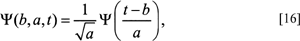
where t refers to the time/boundary domain, a is the scale factor and b is the translation factor. The 1/a term is used for normalization across scales (Costa and Cesar, 2001; see appendix).
Each of these copies are translations and dilations. Specifically, one places the wavelet at the start of the function, f(t), to be decomposed and computes C(1, 1), an amplitude coefficient that determines how closely the wavelet is correlated with the first signal/boundary section. One then repeatedly shifts b-positions to the right and computes C(b, 1), coefficients until one reaches the end of the signal/boundary. One then returns to the beginning of the function, f(t), but now with the wavelet scaled, either dilated or compressed, and computes a new scaled C(b, a) coefficient. One again shifts to the right for increasing b-positions and continues the process of computing C(b, a) amplitude coefficients for each increasing a-scale. In this way, any discontinuity (or singularity) or other changes in curvature along the boundary can be identified.
Another way the wavelet formulation, Eq. [15], can be viewed, is as a measure of the similarity or correlation between the basis function, Eq. [16], and the actual signal/boundary. The coefficients, C(b, a), are a measure of the closeness of the signal/boundary to the wavelet at each scale (Polikar, 1996). It is in this sense that for boundary analysis the wavelet amplitude coefficients can be viewed as measure of change in curvature (see results section). The magnitude of these wavelet coefficients, C(b, a), can be defined as:
where α(b, a) and β(b, a) refer to the real and imaginary parts of the wavelet amplitude coefficients, C(b, a). The complex modulus can then be derived in absolute terms from (see Bolton, 1995, page 147 for details):
and viewed as a matrix of amplitude coefficients. This modulus function can be readily displayed in the Cartesian coordinate system (see results section). If these wavelet coefficients are squared, C(b, a)2, the display of these wavelet coefficients is called a scalogram, which represents the energy distribution, or variance, of the signal. This is analogous to the power spectrum of conventional FDs and EFFs (Antoine et al., 1997).
Of particular importance is the relationship of the scale, the a term in C(b, a), the amplitude coefficients, to the frequency. There is a reciprocal relationship between scale and frequency. Scale, a, is inversely related to the frequency such that 1/a ≅ f, which implies that as the scale values increase, the frequency decreases and visa-versa (Walker, 1999; Costa and Cesar, 2001). The consequence of this critically important relationship will become apparent in the results section.
In one sense, wavelet coefficients are equivalent to those generated with traditional Fourier analysis (FDs). That is, the coefficients, C(b, a), in Eq. [15] can be viewed as amplitude measures in an identical way to the use of the an and bn Fourier coefficients calculated from Eqs. [3] and [4] and used to produce amplitudes (Eq. [5]). In the same vein, the basis functions, Ψ(b, a, t), are analogous to the sin nx and cos nx terms depicted in Eq. [3] and [4]. However, the similarity ends there, as wavelets are localized in both time (or space) and frequency. This is in contrast to sine and cosine waves, which extend infinitely over the interval, [−∞,∞ ] and are incapable of localization in the frequency domain (Olson et al., 1999).
Finally, it should be noted that while the continuous case (CWT) is utilized with the CB data here, the discrete case, DWT, is also often used. An advantage of the DWT is that it eliminates much of the redundancy in terms of very small or zero values of the amplitude coefficients, C(b, a), that computationally arise with the CWT. There are various ways to reduce this redundancy. One approach is to retain only those wavelet coefficients with appreciable magnitude (local maxima). Another one is to calculate the transform skeleton of the CWT (Antoine et al., 1997; Costa and Cesar, 2001).
While a large number of analyzing wavelets are possible, they must satisfy certain constraints to be useful, so only a few have been widely utilized. Some wavelets are more suited to certain applications than to others. Wavelets that have been utilized include the Haar wavelet, originally devised in 1910, Daubechies D4, Morlet, Marr or Mexican hat, Coiflet, etc., For the CB data here, the Mexican hat, a Gaussian-based wavelet function (Antoine et al., 1997; Costa and Cesar, 2001) was utilized as the wavelet of choice (see appendix).
Applications of wavelets include signal processing, the de-noising of data, EEG diagnostics, medical imaging, music and speech synthesis, data and video compression, seismic exploration, feature extraction, computer vision, etc., the list is expanding rapidly (Strang, 1994; Kiltie et al., 1995; Wunsch and Laine, 1995; Wilson, 1999). An example of compression is the now familiar fingerprint data for the Federal Bureau of Investigation (FBI) (Brislawn, 1996). Wavelets are also being used in sedimentology to characterize particle shape. This latter research represents a continuation of work that started with the early application of FDs and FTs (Schwarcz and Shane, 1969; Ehrlich and Weinberg, 1970; Drolon, 1998; Drolon et al., 1999). So far, few applications in biology have utilized wavelets to characterize boundary shape changes. Of three recent papers that have appeared, one (Kiltie et al., 1995) dealt with textural discrimination, another one with growth (Fujii and Matsuura, 1999) from a curve-fitting perspective and a third one (Kashi et al., 1996) with medical diagnosis. Only the last one characterizing the shape of the corpus callosum, is particularly relevant here in terms of shape and shape changes.
If one is primarily interested in shape considerations of form, not just global aspects but also the more localized features, then wavelets become indispensable. This can be justified on the grounds that wavelets: [1] nicely circumvent the difficulty of localization so characteristic of FDs and the FTs, and [2] totally eliminate the subjectivity that arises with EFFs. That is, wavelets provide, for the first time, an objective method that eliminates the unavoidable subjectivity inherent in the selection of landmarks and the use of the centroid distances.
In a schematic fashion, Figure 5 illustrates a two-pronged scenario for combining EFFs with wavelets. One starts with image acquisition from which features of interest are derived. Analysis of the boundary then takes two paths, EFFs are used for the analysis of global aspects of the form, while wavelets are used for the analysis of the localized aspects. As will subsequently be demonstrated, EFFs in conjunction with wavelets, can be considered as a powerful new tool for the quantitative analysis of form. It is this approach that is utilized here.
 View Details | Figure 5. Computational shape analysis utilizes a Fourier-wavelet representation or model. This procedure consists of a dual approach: [1] the computation of FDs, specifically the elliptical Fourier function (EFF), for the characterization of global aspects on the boundary contour and [2] the calculation of the continuous wavelet transform (CWT) for the extraction of localized features (see text). |
This study represents a continuation of our research to delineate the form of the primate cranial base (Lestrel and Moore, 1978; Lestrel and Sirianni, 1982; Lestrel and Roche, 1986; Lestrel et al., 1993). The primary purpose of this study was to explore the presumed stability of the CB in a skeletal series of Japanese skulls (n=297) covering a time frame of over 2,000 years. A secondary purpose was to ascertain the presence of any differences in shape due to sexual dimorphism, differences already discerned earlier in Macaca nemestrina. A two-step approach was utilized to arrive at the above goals. This involved: [1] the use of EFFs to delineate the boundary outline and generate global shape parameters of the CB, and [2] the use of wavelets to discern localized changes in the CB boundary. The use of EFFs was predicated on the fact that they are able to precisely reproduce the outline of 2-D forms, thereby providing an analog of the form. The second step involved in the application of the CWT to the predicted boundary outlines derived from the EFF, so that information about the localization of boundary aspects could be objectively retrieved.
Lateral cephalometric records were available from the Nihon University School of Dentistry at Matsudo, Chiba Prefecture. The cranial data for this study consisted of 297 specimens divided into five archeological age samples. The ages involved in the CB series were from the Yayoi, Kofun, Kamakura, Edo and Modern eras. Although a few specimens where available from the Jomon era (~10,000–300 BC), their questionable condition and small sample size precluded their inclusion in this study. The skulls of the Yayoi, Kofun and Kamakura specimens are from collections housed at Kyushu University, Fukuoka. The Edo specimens are from the National Science Museum, Tokyo, while the Modern samples consisted of students from the Nihon University School of Dentistry at Matsudo.
The Yayoi material comes from two sites: the Doigahama in Yamaguchi Prefecture and the Kanenokuma in north of Kyushu. The Kofun sample comes from cave-type burial sites from both the Tokyo as well as northern Kyushu areas. The Kamakura specimens are largely from the Kanto region. The Edo remains are derived from the Ikenohata site in Tokyo (Details can be found in Ohsako, 2000).
The oldest group, Yayoi (ca. 300 BC–300 AD), consisted of 64 specimens equally divided between females and males. The next group, Kofun (300–593 AD), was comprised of 36 specimens, 16 females and 20 males. The Kamakura sample (1192–1333) consisted of 27 specimens, 17 females and 10 males, while the Edo era (1603–1868) sample contained 64 specimens, 31 females and 33 males. The final group, Modern (ca. 1960+) involved 106 individuals. Of these, 26 were female and 80 were male. All lateral cephalometric radiographs were taken at 70 KV, 50 mA, and an exposure of 0.1 to 0.2 seconds (Ohsako, 2000).
Each radiographic image of the CB was carefully traced onto dimensionally-stable matte acetate sheets using a 0.3 mm lead pencil. The CB on each lateral radiograph was traced starting at basion proceeding along the dorsal clivus to the dorsum sellae, then along the inferior border of the hypophyeseal fossa, continuing anteriorly along the tuberculum sellae to the intersection of the anterior cranial base with the greater wings of the sphenoid (sphenoid registration point-SE). The tracing then continued along the inferior border of the middle cranial fossa to the basilar process and terminating again at basion to create a bounded outline (Figure 6).
 View Details | Figure 6. The cranial base morphology as seen on a lateral radiograph. The contour was carefully traced for each specimen from basion, along the hypophyseal fossa, then anteriorly along the inferior border of the middle fossa to the basilar process, and terminating again at basion. |
A series of points were then precisely located according to a specific protocol (Table 1, Figure 7). Figure 7 illustrates the 54 points used to describe the boundary of the CB. A horizontal line was constructed from basion (point 1, also point 54) to the most inferior aspect of the hypophyeseal fossa (point 20). The distance became Segment 1 or S1. A perpendicular was then constructed from that tangent point (point 20) to create point 43. The horizontal line, from basion to point 20, was then continued anteriorly until it extended past the SE point (point 32). A second vertical line was then extended upward from the SE point (point 32), until it intersected the horizontal line, this marked the limit of Segment 2, or S2. Segment 1, S1, from basion (point 1) to point 20, was then divided into eight equal divisions. These eight divisions were marked and a series of seven vertical lines drawn until they intersected the superior margin of the CB as well as the inferior margin. These intersections generated points 5 to 11 on the superior margin and points 44 to 50 on the inferior margin. In a similar manner, the anterior horizontal segment, S2, from point 20 to point 32, was also divided into eight equal parts. Seven vertical lines were also constructed here until they intersected the superior and inferior margins. These intersections defined points 22 to 28 on the superior margin and points 35 to 42 on the inferior margin. Point 43 is the intersection of a vertical line drawn from point 20. As the areas around basion and SE represented sharp changes in curvature, additional points were added. These additional points were either bisections or trisections. In this way, a set of closely-placed points on the CB boundary has been defined. Some of these points were anatomical landmarks such as basion, while others must be considered as pseudo-homologous points (Sneath and Sokal, 1973). Nevertheless, although these latter points are not strictly homologous, they were precisely located according to the above protocol (Table 1). These points were then labeled on each tracing to keep track of the points during the digitizing step.
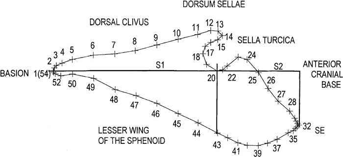 View Details | Figure 7. Plot of the 54 closely-spaced pseudo-homologous points used to describe the cranial base contour. These points were precisely located using a geometrically determined protocol as described in the text (refer to Table 1). |
Each CB tracing was oriented on a 12×12 inch Calcomp digitizer as follows: The center of the digitizer, (0, 0), was carefully identified and marked with a set of crosshairs that extended vertically and horizontally to the edges of the digitizer. Each tracing was placed on the digitizer so that point 20 was superimposed on the origin (0, 0) and the line from point 1 (basion) to point 32 (SE) was made coincident with the horizontal axis of the digitizer crosshairs. The orientation of the CB was with the SE point aligned to the right of the digitizer origin. All 54 points were then digitized clockwise in succession and entered as data to an IBM personal computer with a Pentium III 1.5 mhz processor. Points were subsequently plotted on a Hewlett-Packard HP-6p printer and superimposed on the original tracing to check for errors.
These points were then submitted to a specially written program, EFF23, version 4.0, that computed EFFs for each of the CBs. With 54 points, a maximum of 27 harmonics, subject to Nyquist frequency requirements, were computed. These 27 harmonics were considered more than adequate in terms of fit. The fit with 27 harmonics was checked by calculating the residual or difference between the observed points and the predicted value derived from the EFF. This residual is computed for each point and then averaged over the whole CB. Figure 8 is a computer-generated view to illustrate this curve fit. The dots represent the 54 points and the EFF is shown with a solid line. The mean residual for an individual case is shown as a stepwise procedure. The first harmonic represents an ellipse. With 4 harmonics the residual is 1.71 mm, with 8 harmonics this value drops to 0.67 mm, and with 27 harmonics this value is 0.10 mm for this particular specimen. The mean residual (X±SD) based on a CB sample (n=65) was 0.095±0.014 mm. This value was substantially less than the errors associated with both the tracing and digitizing tasks. The 27 harmonics used to fit the CB, consist of a matrix of 108 separate terms, four coefficients (an, bn, cn and dn) for each harmonic and the two constants (A0 and C0), which need to be computed for each CB (Eqs. [7] and [8]).
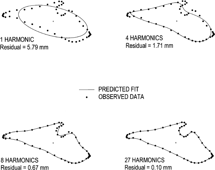 View Details | Figure 8. Computer-generated lateral view of the cranial base outline. The dots represent the 54 observed points. The elliptical Fourier function (EFF) is shown as a solid line and depicted as a stepwise process to display the convergence of the function to an individual observed cranial base outline. As the number of harmonics is added to the series, the fit improves. With 27 harmonics, the average residual was 0.10 mm for this particular specimen. |
Size-standardization was accomplished by scaling all bounded CB outlines so that the area within was a constant 10,000 mm2. Positional-orientation was determined by rotating the major axis of the first ellipse (associated with the first harmonic, shown in Figure 8) so that it was parallel to the horizontal or x-axis as advocated by Kuhl and Giardina (1982).
Since the EFFs closely fit the observed CB, they can be considered as analogs of the actual CB boundary outlines. They were then averaged for each age period (the archeological eras), by sex and plotted. A set of ten sub-groups were involved as there were five age periods and two sexes. These plots were later averaged and superimposed on the centroid to provide a visual assessment of the CB changes with archeological age and sex. These 108-point plots (doubled from 54 to 108 to provide smoother outlines), treated as expected data computed from the EFFs, were used to: [1] generate global shape estimates of the CB, [2] compute distances from the centroid to the boundary, and [3] generate the raw data for wavelet analysis.
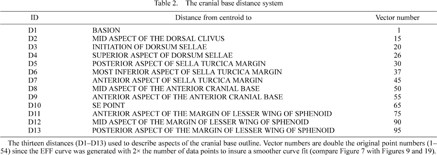
One solution to the inability of identifying local features, characteristic of FDs and FTs, is to use the EFFs in an alternative way. In an attempt to characterize localized aspects along the CB boundary, a set of arbitrary distances were computed from the centroid to selected aspects on the CB margin. These were selected with only one criterion in mind, which was to roughly cover the entire boundary outline. Figure 9 displays the thirteen distances that were chosen (D1–D13). Table 2 provides approximate anatomical definitions of these distances. These bisections between the existing pseudo-homologous points were added to generate a smoother CB margin for visual purposes.
 View Details | Figure 9. The cranial base distance system. The computed set of 13 distances from the centroid to the boundary outline. The number of points has been doubled from 54 to 108 with bisections to insure a smoother outline for visual purposes. |
In an analogous way to EFFs, the wavelet representation used here is also based on a parametric formulation (see Figure 10). This will be made more apparent later. Multi-resolution analysis starts with: [1] a form composed of a set of closely-spaced sampled points on the boundary outline, [2] the calculation of separate x- and y-coordinates (a parametric formulation) which are used to compute the wavelet modulus, C(b, a), and [3] the extraction of significant characteristics (singularities as local maxima, etc., or changes in curvature) in the wavelet frequency domain.
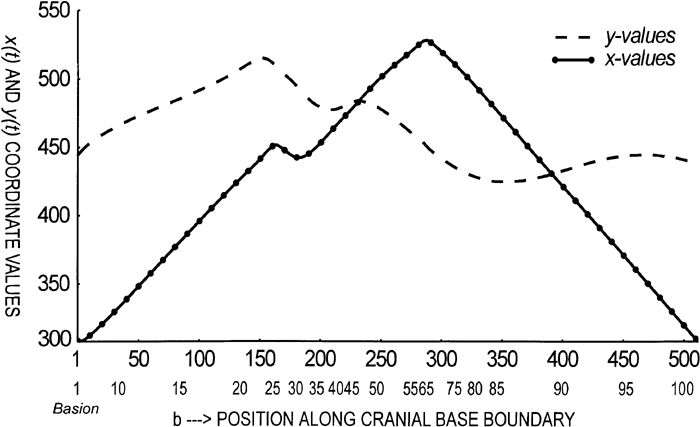 View Details | Figure 10. The parametric formulation required for both the elliptical Fourier function (EFF) and continuous wavelet transform (CWT). The parametrized x(t) curve is shown as a solid line, while the parametrized y(t) one is shown with a dashed line. The y-axis contains the respective coordinate value, x or y. The x-axis refers to either: [1] the 512 evenly divided points along the cranial base outline derived from the CWT, shown as the top row of numbers or [2] the 108 unevenly divided points along the cranial base outline derived from the EFF, shown as the bottom row of numbers (see text). |
Once the size-standardized and positionally-oriented datasets of EFFs have been computed, they were used to generate a set of 108 predicted points. These EFFs were then averaged for each archeological period and for each sex. These averaged 108-point files were then submitted as raw data to a set of Matlab routines that computed the CWT. Prior to computing the CWT, a number of separate steps were required, one of which was that the data has to be set up in parametric form; that is, x and y as function of t (t referring to the position along the CB boundary). This procedure, as well as the others, will be described in more detail below.
The algorithmic procedures involved in the CWT computation, require the utilization of the FFT. Recall that the FFT requires that the CB outline be divided into equal divisions of a power of two. The CB outline was therefore divided into 512 evenly-spaced intervals. What is critical to note here is that initial raw EFF data contains 108 unevenly-spaced points (needed to maintain homology) in contrast to the 512 evenly-spaced points used by the CWT computation. Consequently, it was necessary to map the 108 unevenly-spaced points back into the 512 evenly-spaced points and visa-versa. This was accomplished by running each 108 unequally-spaced data set through a specific routine that generated a new file with 512 equally-spaced points (512 satisfying the power of two requirement), while maintaining a precise mapping of the original 108 points (to the nearest of the 512 points).
However, a caution with this approach needs to be mentioned, in that it is not possible to meaningfully average the 512-point files. There is no problem in averaging the original 108-point files as homology is carefully maintained as these points have been, so to speak, ‘locked’ onto the EFF curve. Consequently, once the evenly-spaced 512-point files are created, any semblance of homology is lost as a function of the equal spacing. For this reason the 512-point files cannot be averaged, the results being meaningless since, again, homology is lost. However, they can be readily created from the averaged 108-point files.
It will be recalled that the EFFs were based on a parametric formulation of the form: x=f(t), y=g(t), In a similar way, a parametric formulation is required for the CWT. It is of the form: u(t)=x(t)+iy(t) (see appendix). Procedurally, this was then carried out on each of the expected point files, recalling that there are now two of them at this stage; the original one with 108 unequally-spaced points and the created one with 512 equally-spaced points. Both files are required. A routine was then created to break each of these expected point files (either the 108 one or the 512 one) into two separate additional files, one containing the x-coordinate and the other the y-coordinate. Thus, four files for each of the ten groups involved (age period and sex) were required. This parametric formulation is displayed in Figure 10.
At this stage one is ready to use the Matlab scripts originally developed by Roberto Cesar Jr. and slightly modified by the senior author. Two scripts were involved. The first one computed the wavelet amplitude coefficients, (or modulus) as a matrix of C(b, a), terms. The second one computed the differences between the mean male and female wavelet amplitude coefficients.
The first script required the 108-point x- and y-coordinate files and the 512-point x- and y-coordinate files respectively, as input (Figure 10). Using these files as data, the second derivative of the Gaussian wavelet was computed (see appendix) and a color plot of the CWT produced, which is intended as a visual display of the wavelet matrix (the modulus values). This color plot, is termed a ‘hot color map’ in that small amplitude values are shown in blue, while larger amplitude values are displayed toward the red, in effect a temperature map (see results) These computed wavelet coefficients were also saved for further analysis with the second Matlab script.
Once the wavelet coefficients were computed and saved, they were then utilized as data in the second script. This script was designed to specifically display the differences observed between females and males. This difference was calculated by subtracting the female matrix from the male one. Two (512×96) matrices of wavelet amplitude coefficients were involved. All color plots derived from the two Matlab scripts, the two initial wavelet plots and the single gender difference plot, were subsequently saved as TIFF files for archiving and future visualization.
‘Computational shape analysis,’ as advocated here, is composed of two elements: [1] measurement of the global aspects of the form and [2] identifying the specific localized entities presumed to be of equal if not greater importance in a biological context. Both global and local aspects are necessary in our attempts to develop a more complete model of form (Figure 5).
Figure 11 and Figure 12 display one approach of deriving global information; namely, the use of a typical amplitude versus harmonic number plot, or as defined earlier, a frequency spectrum. Other global parameters could have also been chosen from the EFF data, such as angulation of the major axes of the computed ellipses, ratio of the major to minor axes, areas of each of the ellipses, etc. The utility of these latter parameters is briefly discussed elsewhere (Lestrel, 2000). Because the EFF is a parametric formulation, the x-amplitude data (Figure 11) and y-amplitude data (Figure 12) have to be viewed separately. As the pattern displayed is basically similar for all age periods, only one group, in this case the Edo age group, is shown here. The remaining plots for the other age periods are not shown, because they are very similar. If desired, they can be obtained from the senior author.
 View Details | Figure 11. Frequency spectrum as percentage amplitude versus harmonic number plot for the mean parametrized x(t) Edo data. Because the first harmonic tends to have an overwhelming effect, it was removed so that the remaining amplitudes could be discerned better. Only amplitudes 2 to 11 are depicted here. Values are in percentages of the total (computed as the sum of the amplitudes for harmonics 1 through 27). Females and males are shown separately (see text). |
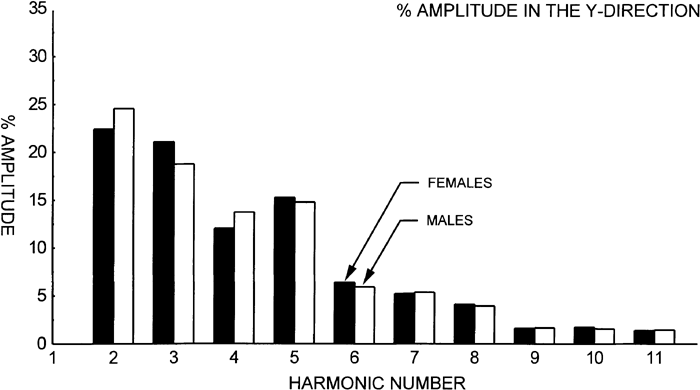 View Details | Figure 12. Frequency spectrum as percentage amplitude versus harmonic number plot for the mean parametrized y(t) Edo data. Because the first harmonic tends to have an overwhelming effect, it was removed so that the remaining amplitudes could be discerned better. Only amplitudes 2 to 11 are depicted here. Values are in percentages of the total (computed as the sum of the amplitudes for harmonics 1 through 27). Females and males are shown separately (see text). |
Because the first harmonic amplitude has an overwhelming effect, as seen in the power spectrum values (explaining over 95% of the variance in the x-direction and 92% of the variance in the y-direction for this data) it tends to swamp the effect of the higher terms. For this reason, it was excluded so that the remaining amplitudes could be discerned better. Finally, it should be noted that for both Figure 11 and Figure 12 the mean percentage amplitude values are a function of the total, which is the sum of harmonics 2 through 27.
While there are differences between males and females for the Edo group, these differences are quite moderate and tend to be somewhat random in character. It is important to note that each of the harmonic amplitudes from 2 to 11 is contributing an aspect to the total form. However, these morphological CB aspects measured by the amplitudes are global in nature. In other words, the effect of each amplitude is spread out, or smeared as mentioned earlier, over the whole CB boundary outline. If there were any localized differences between the male and female samples, (and one can safely assume that there are) this method would not detect them. Thus, while amplitudes can be considered appropriate measures for estimating global aspects of form, they are largely useless for identifying localized features. For those aspects we have to turn to other approaches.
One such approach consisted of choosing selected distances from the centroid to aspects of interest on the CB contour (Figure 9, Table 2). Utilizing the thirteen distances (D1–D13), a correlation matrix was calculated to reduce the appreciable correlation among the variables. Variable pairs with correlations equal to or greater than 0.8 had one variable removed leaving seven out of the original thirteen. These seven were then analyzed utilizing a two-way MANOVA with two ‘group-effects’, archeological age and sex. Table 3 displays the MANOVA table showing the two ‘between-group’ contrasts: type (five archeological age groups) and sex (female versus male). These data are size standardized (i.e., shape only) and positionally oriented (insuring a common orientation in space). As statistically significant differences were found for both age and sex, this allowed for the further computation of univariate F-tests. Table 4 shows the univariate F-tests for both contrasts: group and sex. For the type contrast, distances D1, D2, D3 and D4 were statistically significant and for the sex contrast, D2, D4, D7 and D12 were significant. However, since the presence of significant systematic differences for sex was based on a set of subjectively chosen distances, this prompted a re-examination using wavelets.
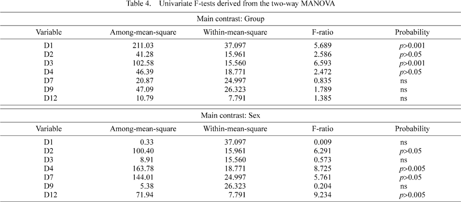
To alleviate the inevitable subjectivity in the choice of measurements as seen with EFFs, wavelets were utilized. The following figures have been embedded in a Cartesian ‘position-scale’ plane with the vertical axis representing the scale levels and the horizontal axis displaying the position along the CB boundary contour.
Figure 13 displays a 3-D plot of the Yayoi mean female data. The position along the CB boundary is shown on the x-axis, while the scale values are on the y-axis. The scale axis starts with level 1 (highest frequency) and ends with level 96 (lowest frequency). The amplitude or modulus values (absolute wavelet coefficients) are depicted on the z-axis. Note that the wavelet amplitude values are quite small at level 1 (~0.00–0.08) and show a 100-fold increase by level 96 (~1.00–8.00).
 View Details | Figure 13. A 3-D plot of the continuous wavelet transform (CWT) for the mean Yayoi female data. The y-axis depicts scale levels 1 through 96 (every 10th one). The x-axis shows the position along the CB contour and the z-axis displays the wavelet amplitude coefficients derived from the CWT. Note that the CWT wavelet magnitude values for the scale levels, from the smallest (level 1) to the largest (level 96), differ by a factor of 100. |
Figure 14 is an ‘enlarged’ scale plot of the female Yayoi data, but now limited to level 1 and level 96. Local discontinuities (singularities) are now clearly delineated with level 1. Maximal wavelet values are associated with points 1, 25 and 63, which reflect the sharpest changes in the curvature along the CB contour. However, by level 96, this precise localization is largely lost, although the major or gross shape changes in the CB contour are being maintained. Note that while the major peaks associated with level 96, approximate those seen with level 1, their position along the CB boundary is now imprecise. This figure clearly shows that as the CWT begins to increasingly blur the precise locations on the CB contour at larger scale values, acting in analogous way to a smoothing function, only some of the curvature information is still being retained.
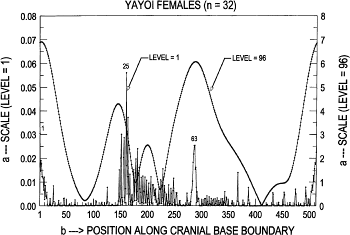 View Details | Figure 14. An enlarged 2-D plot for Yayoi female data. Displayed here is the continuous wavelet transform (CWT) with just two scaling levels. The amplitude values for level 1 are on the left y-axis. The amplitude values for level 96 are on the right y-axis. Level 1 represents a depiction of the high frequency components along the CB contour, while level 96 shows the low frequency components. Maximal wavelet values are identified for points 1, 25 and 63, reflecting sharp shape changes in the curvature of the CB contour (see text). |
Figure 15 illustrates the CWT as a color plot for the mean female Yayoi group. As before, the CWT was computed as a matrix of modulus values or wavelet coefficients, Eq. [18], each matrix containing 96 levels (scale) by 512 positions, or 49,152 element values. The 512 positions along the horizontal or x-axis have now been mapped back into the 108 unevenly-spaced points on the CB boundary as discussed earlier. The 96 levels determining the scale are shown on the vertical or y-axis. This figure has been embedded in a Cartesian ‘position-scale’ plane with the vertical axis representing the scale and the horizontal axis the position along the CB boundary. This plot can be thought of as looking down onto the x-y plane (scale-position plane) of Figure 13, but with the amplitude wavelet values (z-plane) now embedded (or compressed) into the x-y plane.
 View Details | Figure 15. Continuous wavelet transform (CWT) of the mean Yayoi female data. The y-axis refers to the scale (96 levels) and the x-axis represents the position (108 points) along the cranial base boundary. Color is now used to identify the magnitude of the wavelet coefficients. Dark blue indicates regions of low wavelet amplitude value, while red indicates areas of high amplitude value. Particularly high values can be found at points 1, 25, 31, and 63, identifying regions of high curvature. Note: The 512 points cranial base points have been mapped back into the 108 points (see text). |
For visibility, these amplitude values have been identified with color, with the high frequency components in blue, and the low frequency components in red. Color is used here to indicate the strength of the signal. The ‘signal’ in this case can be viewed as a measure of the curvature along the CB margin. While the best resolution of the localized changes in curvature are depicted with level 1, the actual magnitudes of the CWT amplitude values at that level are rather low (~0.00–0.08), hence the blue end of the color spectrum. In contrast, if we look at highest computed scale level, level 96, the amplitude values are substantial (~1.00–8.00), and are therefore mapped into the red end of the color spectrum. It should be noted that while the strongest wavelet signals (for each scale level) are around points 1, 25 and 63, which show strongly in the red part of the spectrum, it is at the blue end of the spectrum (top of Figure 15) that the localization is the most precise (reference should to be made to Figure 13 and Figure 14 to facilitate an understanding of Figure 15).
Figure 16 displays the 3-D plot of the mean Yayoi male data. The pattern is very similar to that of the Yayoi female data. On closer scrutiny one can detect slight differences in the curves depicting the scale levels. An ‘enlarged’ scale plot of the male Yayoi data, again limited to level 1 and level 96 is shown in Figure 17. The pattern is again very similar to that of the female Yayoi data, although, on closer analysis, minor differences can be observed.
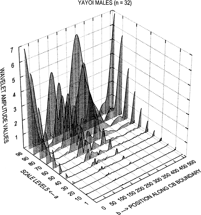 View Details | Figure 16. A 3-D plot of the continuous wavelet transform (CWT) for the mean Yayoi male data. The y-axis depicts scale levels 1 through 96 (every 10th one). The x-axis shows the position along the CB contour and the z-axis displays the wavelet amplitude coefficients derived from the CWT. Note that the CWT wavelet magnitude values for the scale levels, from the smallest (level 1) to the largest (level 96), differ by a factor of 100. |
 View Details | Figure 17. An enlarged 2-D plot for Yayoi male data. Displayed here is the continuous wavelet transform (CWT) with just two scaling levels. The amplitude values for level 1 are on the left y-axis. The amplitude values for level 96 are on the right y-axis. Level 1 represents a depiction of the high frequency components along the CB contour, while level 96 shows the low frequency components. Maximal wavelet values are identified for points 1, 25 and 63, reflecting sharp shape changes in the curvature of the CB contour (see text). |
Figure 18 displays the CWT as a color plot for the mean male Yayoi group. Again, the wavelet amplitude values have been identified with color; that is, the high frequency components are blue, while the low frequency components are in red. The overall pattern is very similar to that of the mean female Yayoi group, although on closer analysis, minor differences can be discerned. It is these differences that are of biological interest and will be taken up subsequently.
 View Details | Figure 18. Continuous wavelet transform (CWT) of the mean Yayoi male data. The y-axis refers to the scale (96 levels) and the x-axis represents the position (108 points) along the cranial base boundary. Color is now used to identify the magnitude of the wavelet coefficients. Dark blue indicates regions of low amplitude value, while red indicates areas of high amplitude value. Particularly high values can be found at points 1, 25, 31, and 63, identifying regions of high curvature. The 512 points cranial base points have been mapped back into the 108 points (see text). |
To appreciate the significance of these wavelet amplitude plots, especially the ones in color (Figure 15 and Figure 18), it is important to understand the relationship between the scaling values (the ‘a’ along the y-axis) and the frequency. Recall that scale, a, is inversely related to the frequency (1/a ≅ f). This indicates that as the scale values (levels) increase, the frequency will decrease. Consequently, when viewing Figure 15 and Figure 18, one needs to keep in mind that the amplitude values (modulus) dealing with the position along the CB outline (the ‘b’ along the x-axis) associated with the highest frequency, are at the top of each plot. That is where the scaling value (level), a, is the lowest. In contrast, the lowest frequencies are at the bottom of each plot. This is where the scaling value, a, is the highest. Moreover, these low frequency components (shown largely in red) are, ‘blurred’, or more spread out along the horizontal axis (this is clearly depicted in Figure 14 and Figure 17). These low frequency components are characterizing aspects of the CB that are now less localized and cover more of the morphology. In other words, they are better at detecting structural homologies in contrast to point homologies, which have more in common with singularities. The low frequency components describe the more gradual changes in the CB contour, making them perhaps conceptually closer to the notion of homology as originally proposed by Owen in 1843.
While all this may be somewhat counter intuitive when one is viewing these wavelet plots, it is completely in accord with the results from conventional FDs as well as EFFs. The low frequencies are responsible for the more global aspects of form, while the higher frequencies are responsible for the smaller localized features on the boundary of the form, even if the precise locations of those features cannot be readily identified in the frequency domain using FDs and FTs.
A particularly illustrative example of this relationship between scale and frequency, using 2-D wavelets, can be seen in Hubbard (1998, page 235). Which frequencies are more important? The answer depends on the application. Both frequencies, the high and low, and possibly even middle values may provide valuable information and be of importance in computational shape analysis.
Recall that the wavelet is particularly sensitive to the presence of singularities and/or changes in curvature. This is now clearly reflected in the CB boundary for the Yayoi data. The highest frequencies are associated with what could be roughly identified as singularities as seen at point 1 (basion) and at point 63 (SE), regions of sharp curvature, while somewhat lower frequencies cover ranges of points that describe regions with more gradual changes in curvature, such as around points 22 to 27 (dorsum sellae), points 29 to 40 (sella turcica) and points 45 to 47. What is particularly important to recognize here is that these locations on the CB boundary were identified and numerically described (maximal values of the amplitude coefficients or modulus values) in a totally objective manner.
Figure 19 shows the centroid-superimposition of the mean female Yayoi group (solid line) on the male Yayoi group (dotted line) for the area-standardized and positionally-oriented data derived from the EFFs. While there were minor differences present in the superimposition of the Yayoi gender plots, the anterior displacement of the male trace in contrast to the female one, at the posterior aspect of the hypophyeseal fossa, was particularly apparent. This systematic anterior displacement was seen in all groups-Kofun, Kamakura, Edo and Modern periods- and is of particular biological interest. This difference in sexual dimorphism was further examined by subtracting the mean male CWT amplitude coefficients from the mean female CWT coefficients.
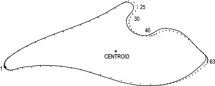 View Details | Figure 19. Size-standardized and positionally-oriented cranial base (CB) superimpositions. Plot of the centroid-based superimposition of the mean Yayoi female (solid line) trace on the mean Yayoi male (dotted line) trace. Note the anterior displacement of the dorsum sellae aspect of the males with respect to females. |
In a similar way to Figure 14 and Figure 17, Figure 20 displays an enlarged plot of the mean gender differences in the CWT, again limited to scaling levels 1 and 96. As can be seen from Figure 19, the major difference between males and females takes place around point 25, the anterior aspect of dorsum sella. The localization is well documented with the high frequency component (level 1). The picture, however, is not so clear-cut at the lowest frequency component (level 96), which seems to display other more spurious elements (noise) along the CB boundary as well.
 View Details | Figure 20. An enlarged 2-D plot showing Yayoi sexual dimorphism. Displayed here is the continuous wavelet transform (CWT) with just two scaling levels. The amplitude values for level 1 are on the left y-axis. The amplitude values for level 96 are on the right y-axis. Level 1 represents a depiction of the high frequency components along the CB contour, while level 96 shows the low frequency components. Maximal wavelet values are present for point 25, reflecting the major area of difference in curvature of the CB contour between the mean male and female outlines Note that the CWT wavelet magnitude values for the scale levels, from level 1 to level 96, now differ by a factor of 10 (see text). |
Figure 21 displays the difference CWT plot. One can now see that the major differences between the mean female Yayoi group and the mean male Yayoi group are concentrated around points 25 to 30 (hypophyseal fossa), and to a considerably lesser degree around points 42 to 45. This pattern is generally in accord with Figure 19. As a caveat, it must be mentioned that the centroid superimposition (Figure 19) is slightly different (it is not a least-squares approach that effectively minimizes the differences) from the results of the subtraction (Figure 20), so while quite close to the results displayed with the CWT difference plot, it is not exact.
 View Details | Figure 21. Continuous wavelet transform (CWT) differences. Sexual dimorphism between mean Yayoi females and mean Yayoi males is depicted here. The y-axis refers to the scale (96 levels) and the x-axis represents the 108 points along the cranial base boundary. Color is used to identify the magnitude of the wavelet coefficients. Dark blue indicates regions of low value, while red indicates areas of high value. High values are present in the region defined by points 25 to 30. These points correspond to the largest difference between the male and female traces (refer to Figure 19). The 512 points cranial base points have been mapped back into the 108 points (see text). |
Results for Kofun, Kamakura, Edo and Modern periods are not shown, simply because they are very similar to those of the Yayoi and would take up too much space here. If desired, interested parties can get the results for all groups from the senior author.
The numerical description of the shape of complex and irregular 2-D morphological forms continues to present challenging issues that need to be resolved. Earlier approaches, such as EFFs, represent one of the advances developed for quantitatively characterizing the contour of complex morphologies of the type encountered in the biological sciences.
The computational shape analysis model advocated here, with the Fourier-wavelet representation, is based on an approach that partitions the shape of a form (defined as the boundary or contour) into two aspects: global elements and local features. To be able to analyze these two aspects, two techniques need to be joined. These are the utilization of EFFs and the application of CWTs. The initial use of the EFFs is to generate invariance with respect to: [1] starting point, [2] maintenance of point homology, [3] standardization for size and [4] positional orientation. In addition, EFFs produce a precise analog of the morphology under consideration, difficult to generate with other methods. Once this analog of the form has been created, EFFs can then be subsequently used to compute amplitudes, phase, power, and a host of other measures, which are all global estimates of the shape of interest.
However, these global estimates are incapable of deriving any information about localized elements on the contour of the form. In particular, the presence of singularities or rapid changes in the curvature of the boundary is missed with these global parameters. This has been a serious limitation with Fourier analytic methods since their inception. The need to circumvent this restriction has led to alternative procedures, one of which has been to use EFFs for the computation of distances from the centroid to the boundary. While useful, this approach has the undesirable drawback in that these measures are subjectively chosen. What is required is a methodology that identifies these changes in boundary curvature in a completely objective fashion. The comparatively recent development of CWTs finally provided the solution.
Recall that the wavelet is particularly sensitive to the presence of singularities and/or changes in curvature. This was clearly reflected in the CB boundary for all age groups from the Yayoi to Modern. The highest frequencies are associated with what could be roughly identified as singularities as seen at point 1 (basion) and at point 63 (SE), regions of sharp curvature. Another region with considerable curvature changes is at point 31. The lower frequencies cover ranges of points that describe regions with more gradual changes in curvature. For example, around points 22 to 27 (dorsum sellae), points 29 to 40 (sella turcica) and points 45 to 47. It is particularly important to recognize that these locations on CB boundary were identified and numerically described (maximal values of the wavelet amplitude coefficients or modulus values) in a totally objective manner.
Two conclusions can be drawn about the current study of the human CB: [1] although group differences were present, they seemed to be quite small and largely random in character, suggesting the presence of considerable stability in the CB structures over time; and [2] the presence of systematic differences between female and males. This latter conclusion is consistent with earlier data derived from studies of sexual dimorphism in Macaca nemestrina (Lestrel and Moore, 1978; Lestrel and Sirianni, 1982; Lestrel et al., 1993). In the current study, these differences in sexual dimorphism were present for every group starting with the Yayoi period and continuing up to the Modern period. Consequently, one may infer that the pattern of sexual dimorphism documented in the Japanese CB, is a primate pattern with an ancient evolutionary history.
As demonstrated here, wavelet analysis is particularly useful for the objective identification of major (and presumably of biological significance) local features, difficult if not impossible to identify easily with other methods, including conventional FDs and FTs. The Fourier-wavelet model allows for a more comprehensive numerical representation of the shape and thus, able to quantify more completely the visual information that is so readily observable in the biological world around us.
As senior author, I wish to thank my colleague Roberto M. Cesar Jr., of the University of Sao Paulo, Brazil, for his generous help with wavelets, for providing me with the Matlab scripts so that I could compute the wavelets myself as part of the learning process and for critically reviewing the manuscript. I am especially indebted to Prof. Yuji Mizoguchi, Department of Anthropology, National Science Museum, Tokyo, for his kindness in allowing me to participate in his session at the IUAES 2002 meetings. I also wish to thank Prof. Eisaku Kanazawa, Department of Anatomy, Nihon University School of Dentistry at Matsudo, Chiba, and Prof. Fumio Ohtsuki, Emeritus, Tokyo Metropolitan University, Hachioji, for encouraging my attendance at the conference. I especially wish to thank Dr. Osamu Takahashi, formerly at the Nihon University School of Dentistry at Matsudo, Chiba, now in private practice, for his generous assistance with the lateral radiographs of the cranial base data housed there. Special thanks also go to Dr. Neal Garrett, UCLA School of Dentistry, Dr. Albert Bodt, Kaiser Permanente, and Paul Scardino of Western Vision Software, Layton, Utah, for reviewing the manuscript. Thanks also go to my wife, Dagmar, whose talents as a librarian were, as usual, helpful. I am especially grateful to Charles Wolfe, my longtime colleague, for his programming efforts, with both EFFs and the Matlab scripts, and also for reviewing the manuscript. Any errors remaining are solely my own. We gratefully acknowledge the research support of grants FAPESP (99/12765-2) and CNPq (300722/98-2) to R. Cesar Jr. F. Finally, we wish to thank the anonymous reviewers for their constructive remarks. The interested reader can obtain the software (EFF23) used in part for the preparation of this paper at a nominal cost from the senior author. A Microsoft Windows version (MLmetrics), which is an expanded version of EFF23 is in preparation.
|