| Edited by Fumio Tajima* Corresponding author. E-mail: hideki.innan@uth.tmc.edu |
A substantial fraction of the eukaryotic genome consists of duplicated genes or chromosome segments (Lynch and Conery 2000; Bailey et al. 2002). Gene duplication has been considered as a primary source for adaptive genome evolution because one copy has a great opportunity to acquire a new novel function while the other copy keeps the original function (neofunctionalization) (Ohno 1970). However, it is not clearly understood how often neofunctionlization occurs because one of the duplicated genes is likely to be silenced (nonfunctionalization) relatively quickly after duplication (Li 1980, Lynch and Conery 2000). Thus, the fates of duplicated genes have been under extensive debate for a long time (e.g., Ohta 1987; Walsh 2003).
To address this question, it is important to study the evolutionary mechanism in early stages of duplicated genes, where the fate of duplicated genes is likely to be determined. In this article, I review the recent development of theories for analyzing single nucleotide polymorphism data in young duplicated genes, where concerted evolution via gene conversion is going on. Concerted evolution is a unique evolutionary phenomenon for multigene families where copy members of a family evolve in a non-independent manner (Ohta 1980; Dover 1982, Arnheim 1983, Li 1997). That is, copy members exchange sequence information with each other so that the sequence divergence among the members of a multigene family is maintained low. Mechanisms such as intergenic (i.e., non-allelic) gene conversion and unequal cross-ing-over should be involved. Gene conversion is considered as a primary mechanism for concerted evolution of small multigene families because it explains the homogenization of genetic variation between copy members without changing the number of copies in a family (e.g., Ohta 1983; Li 1997).
Fig. 1 illustrates a possible realization of the behavior of the level of divergence between duplicated genes after gene duplication (Teshima and Innan 2004). The divergence first increases and reaches an equilibrium, which is determined by the balance between mutational input of variation and homogenization by gene conversion. Then, the level of divergence fluctuates around its equilibrium value for a while. The two duplicates are under concerted evolution in this time period. In this review, we consider how to understand and analyze DNA polymorphism (SNP) data in a pair of duplicated genes under concerted evolution. During concerted evolution, the pattern of polymorphism is complicated because gene conversion transfers polymorphism in one gene to the other creating ‘‘shared polymorphic sites” at which polymorphism is observed at the paralogous sites in both genes. A number of shared polymorphic sites are observed in duplicated genes; examples include several pairs of duplicated genes in Drosophila (Inomata et al. 1995; King 1998; Lazzaro and Clark 2001; Bettencourt and Feder 2002), human (Innan 2003b), plants (Sato et al. 2002; Charlesworth et al. 2003) and Plasmodium falciparum (Neilsen et al. 2003).
 View Details | Fig. 1. Illustration of the behavior of the divergence between duplicated genes, modified from Teshima and Innan (2004). |
Concerted evolution does not continue forever as illustrated in Fig. 1. Concerted evolution might be terminated when the two duplicated genes happen to escape from gene conversion (Walsh 1987; Innan 2003b). Selection resulting in neofunctionalization is one of the causes to terminate concerted evolution, although others include neutral mutations (insertion/deletions and accumulation of nucleotide mutations) that works as a barrier against gene conversion. In this review, we also consider how selection works at the end of concerted evolution. Once the two duplicated genes successfully escaped from gene conversion and got diverged at a certain level, they are not subject to homogenization any more and DNA polymorphism data in each gene can be analyzed independently.
Fig. 2 illustrates an example of a pattern of DNA polymorphism in a pair of duplicated genes, I and II, under concerted evolution. Suppose that six haploid individuals are resequenced for both of the duplicated genes. Based on the alignment of the 12 sequences, ten variable (segregating) sites are detected. These sites are classified into three categories: (i) Shared polymorphic sites, at which polymorphism is observed in both of the two genes. (ii) Fixed sites, at which each gene has a different fixed nucleotide. (iii) Specific polymorphic sites, at which polymorphism is observed in either of the two genes. Blue, red and yellow lines in Fig. 2 represent these three classes of sites, respectively. The first type of polymorphic sites (shared polymorphic sites) are a characteristic of polymorphism in a pair of duplicated genes, and could be strong evidence for gene conversion given the mutation rate per site is low.
 View Details | Fig. 2. An example of polymorphism data in duplicated genes, I and II. Mutations that occurred in genes I and II are represented by pink and green boxes, respectively. |
For each biallelic segregating sites with A and a, we can calculate the following amounts of variation:


where n is the total number of haploid individuals (n = 6 in this example) and nxy is the number of haplotypes with nucleotide x in gene I and y in gene II (x and y represent two segregating nucleotides at the focal site and ‘‘–’’ can be either A or a). hw1 and hw2 are the heterogeneities in genes I and II, respectively, which are identical to heterozygosities per site. hb is the heterogeneity between two genes, which is the probability that two randomly chosen alleles from two genes (excluding those on a single haploid individual) are different. D is the level of linkage disequilibrium, whose bias due to finite sample size is adjusted (Innan 2002). In Fig. 2, hw1, hw2, hb and D are shown for each of the ten segregating sites. It is obvious that these four values are zero at non-segregating sites.
When we look at the whole genes together, it is more reasonable to consider the amounts of variation per gene, which can be given by


where L is the total number of nucleotides in each gene. hw(k), hb(k) and D(k) represent hw, hb and D at the kth site, respectively. Equation 5 can be used for both πw1 and πw2. Equation 5 is identical to the average numbers of pairwise nucleotide differences within each gene, which are calculated by

for each gene, where d11(i, j) and d22(i, j) represent the observed numbers of nucleotide differences between the ith and jth haploid individuals for genes I and II, respectively. πb is identical to the average number of pairwise nucleotide differences between two genes, which is written as

where d12 (i, j) represents the observed number of nucleotide differences between gene I on the ith haploid individual and gene II on the jth haploid individual. Note that this equation does not consider the differences between two genes on the same haplotype as well as Equation 3. In the following sections, simple theoretical models are considered to obtain the expectations of these amounts of polymorphism.
In this section, a simple two-allele model for a single pair of nucleotide sites in duplicated genes (Innan 2002) is considered. Since mutation rate per nucleotide site is very low, the two-allele model is a reasonable approximation for modeling nucleotide polymorphism (Kimura 1969). This model is the simplest case of Ohta’s multiple-allele multiple-locus model (Ohta 1982). Ohta (1982) obtained allelic identity coefficients by using complicated transition probability equations. Here, the two-locus two-allele model is simple enough to use a diffusion equation, which is more flexible than the transition probability equations, especially when selection is incorporated.
The model represents a particular pair of nucleotide sites in duplicated genes, I and II, each of which consists of L nucleotides as shown in Fig. 3. We consider two neutral alleles, A and a, so that there are four possible haplotypes, A-A, A-a, a-A, and a-a, where the first character is the allele at gene I and the second is for gene II (Fig. 3B). The frequency of these four haplotypes are denoted by x1, x2, x3, and x4, respectively. The model considers mutation, gene conversion and recombination in a finite-size diploid population with a constant size N. Mutation occurs between two alleles at a rate μ per generation. Gene conversion changes A-a and a-A to A-A at rate c per generation, and to a-a at the same rate. Let the recombination rate between two sites be r per generation. Then, the expected frequencies of the four haplotypes in the next generation are given by
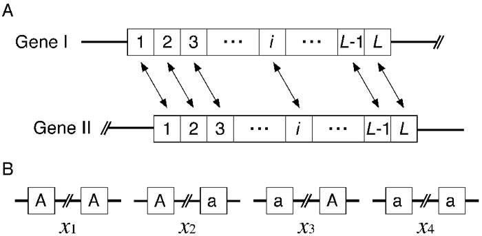 View Details | Fig. 3. (A) Illustration of the two-gene model for duplicated genes. (B) Two-site model for a single pair of nucleotide sites in duplicated genes. Four possible haplotypes are shown. |


where D = x1x4 – x2x3, the linkage disequilibrium in the population. Note that (4) gives an estimate of D from the sampled individuals.
Based on these recursion formulas, a diffusion method (Kimura 1964; Ohta and Kimura 1969b) is employed to obtain the expectations of hw, hb and D. Here, we define another two parameters, p and q, which are the frequencies of A in genes I and II, respectively:

Then, from Equations 11–15, we can construct a three-dimensional diffusion equation. That is, g = g(p, q, D), an arbitrary function of p, q and D satisfies the following equation at equilibrium:

where

(Innan 2002), where θ = 4Nμ, C = 4Nc and R = 4Nr. When there is no gene conversion (i.e., C = 0), this equation is identical to equation (12) in Ohta and Kimura (1969a).
From Equation 16, we have the expectations of hw, hb, and D at equilibrium:


where


(Innan 2002).
The model assumes there are L pairs of two-locus (sites) models in duplicated genes I and II (Fig. 3). Therefore, it is straightforward to obtain the expectations of the amounts of DNA variation per gene under the finite-site model:


When L is large and the mutation rate per site is very low, it is reasonable to assume the infinite-site model (Kimura 1969), where the expectations of πw, πb and Dsum are obtained from Equations 24–26 by letting L infinity with Θ = Lθ constant:


In Fig. 4, E(πw), E(πb) and E(Dsum) are plotted. Given that E(πw) = 1 in the regular single-locus model because Θ = 1 is assumed, the top panel shows that the expected level of polymorphism is higher (at most twice) in a duplicated gene than a single-locus gene in which E(πw) = Θ. E(πb) decreases with increasing the gene conversion rate. E(πb) is an increasing function of the recombination rate, indicating recombination improves the efficiency of homogenization. Gene conversion makes positive linkage disequilibrium because of an excess of A-A and a-a haplotypes. As R increases, E(Dsum) decreases.
 View Details | Fig. 4. Expectations of πw, πb, and Dsum. Θ = 1 is assumed. |
Since E(πw), E(πb) and E(Dsum) are given by simple functions of Θ, C and R, we can estimate Θ (or θ), C and R from (27), (28), and (29). That is,


With the example data of Fig. 2, Θ, C and R are estimated to be 1.91, 0.565 and 2.75, respectively, given πw = (3.05+2.85)/2 = 2.95, πb = 4.8 and Dsum = 0.43.
The equations are also applied to the polymorphism data of the distal and proximal amylase genes in Drosophila melanogaster (Araki et al. 2001). Both genes are located on chromosome 1 with a short intergenic region (≈ 4.5 kb). In the Kenyan sample (n = 10), 78 variable sites are detected in the alignment of the total 20 sequ-ences, of which 37 are shared polymorphic sites. Fig. 5 summarizes these sites with their ancestral states estimated from D. simulans, although the estimates might not be very reliable because of quite high divergence between the two species (Innan and Tajima 1997). The three amounts of variation are calculated to be πw = 20.40, πb = 22.04 and Dsum = 2.72. Then, we estimate Θ = 12.92 θ = 0.0087), C = 4.55 and R = 22.99. The estimate of the gene conversion rate is about 500 times larger than that of the mutation rate, indicating this high rate of gene conversion has created the observed many shared polymorphic sites. The estimate of the mutation parameter (θ = 0.0087) is in a typical range for this species.
 View Details | Fig. 5. Polymorphism in the Kenyan sample (n = 10) in the proximal and distal Amy genes of D. melanogaster. Data from Araki et al. (2001). Shared polymorphic sites are shown in blue. |
Although the simple model considered above provides exact analytical results, it is also very important to develop a tool to simulate patterns of DNA polymorphism to study variable stochastic processes in a population. This makes it possible to test whether an observed pattern is consistent with a neutral model. In this section, a coalescent algorithm to simulate patterns of polymorphism in duplicated genes with intergenic gene conversion is introduced (Innan 2003a).
Consider a pair of duplicated genes that are at equilibrium (i.e., we assume that the number of genes is two for a very long time). For simplicity, it is also assumed that recombination occurs only between two genes, although intragenic recombination is easily incorporated (e.g., see Nordborg 2001). To simulate gene conversion bet-ween two duplicated genes, the standard coalescent with recombination (Hudson 1983) is modified. Fig. 6 illustrates an example of an ancestral recombination graph of a pair of duplicated genes for n = 3, which is generated backward in time. All lineages are shown by double lines, the left is for gene I and the right is for gene II. Under the framework of the coalescent, two events, coalescent and recombination occur at rates 1/2N and r per generation, respectively. Two lineages merge by a coalescent event, and the double lines of a lineage are separated by a recombination event. Simultaneously, gene conversion is also simulated, which occurs at rate c per site per generation. For each gene conversion event, the position and direction are determined. The distribution of the length of gene conversion tracts may be approximated by a geometric distributions (Wiuf and Hein 2000; Teshima and Innan 2004). For convenience, the gene is represented by an interval of (0, 1), so that the position of a gene conversion tract is given by an interval between 0 and 1.
 View Details | Fig. 6. A possible realization of an ancestral recombination graph with gene conversion for n = 3, from Innan (200a). The filled circles represent mutations and the two open circles are the MRCA for the two genes. Gene conversion events are represented by arrows. For example, the left-headed arrow between T0 and T1 means that gene conversion transfers a fragment in the interval (0.08–0.27) from gene II to gene I. |
There are two major modifications here: (1) Lineages that are not ancestors of the sampled chromosomes are also traced. Such lineages are shown in broken lines in Fig. 6. (2) The simulation continues until the whole simulated region reaches the Most Recent Common Ancestor (MRCA) of the two genes, which is usually much older than the MRCA of each gene. The lineages of two different genes can reach their MRCA by gene conversion. That is, gene conversion works essentially as a coalescent event between two paralogous genes. The detailed procedure of the coalescent simulation is described in Innan (2003a), and a simulation code is available on request from the author.
This coalescent simulation is very powerful to study the pattern of polymorphism. For example, Fig. 7 shows the expected allele frequency distributions of three categories of polymorphic sites obtained by coalescent simulations. When the gene conversion rate is low (C = 0.2), a number of fixed sites are observed and specific polymorphic sites are much more than shared polymorphic sites. As C increases, fixed sites decreases and most polymorphic sites are shared by the two genes.
 View Details | Fig. 7. Expected allele frequency distributions. R = 10 is assumed but the effect of R is relatively small, from Innan (2003a). |
Tests of neutrality based on the allele frequency spectrum can also be performed by a coalescent simulation. Fig. 8 shows the observed spectra in the distal and proximal Amy genes of D. melanogaster. They are similar to the expected spectrum obtained from a simulation given the estimated values of Θ = 12.92, C = 4.55 and R = 22.99, indicating a neutral model can explain the observation very well. This is consistent with the result of Tajima’s D test (Tajima 1989). For the distal and proximal Amy genes (polymorphisms in the two genes are analyzed separately), Tajima’s D is calculated to be –0.13 and 0.10, respectively. These D values are not significantly different from 0 when the null distribution of D is obtained from a simulation with 10,000 replications with the estimated parameters, Θ, C and R.
 View Details | Fig. 8. Observed allele frequency distributions in the Amy genes in D. melanogaster with the expected distribution, which is obtained from coalescent simulations with the estimated parameters (Θ = 12.92, C = 4.55 and R = 22.99). From Innan (2003a). |
It is interesting to note that Tajima’s D test works to detect purifying selection, which makes the D value negative. However, a regular balancing selection with two ancient alleles can not be detected by Tajima’s D test in duplicated genes with gene conversion. In a single locus system, two ancient alleles maintained by balancing selection creates a positive D value. On the other hand, this type of selection works in a different way in a two locus system.
Consider two such alleles, A and B. Assume that individuals with both alleles are advantageous over those with only one allele. In a single-locus system, a diploid individual can have the two alleles as a heterozygote, so that only up to half the individuals in a population can be advantageous. However, in a two-locus system, all individuals (even haploids) can have the two alleles. That is, A in one locus and B in the other (i.e., ‘‘permanent heterozygote’’ Spofford 1969).
This permanent heterozygote is a very attractive way to maintain two different alleles in duplicated genes, and it should be an initial stage to lead to neofunctionalization. However, gene conversion is an enemy of permanent heterozygote because it homogenizes the allelic state. That is, the ‘‘heterozygote” haplotype, A-B and B-A, could be homogenized to A-A and B-B by gene conversion. This means that A-B and B-A are not permanent heterozygotes under the pressure of gene conversion. To keep the two alleles, strong selection to favor A-B and B-A over A-A and B-B is necessary. This evolutionary battle between selection and gene conversion is modeled by (Innan 2003b), in which the relative fitness of A-B and B-A is given by 1 and that of A-A and B-B is given by 1-s. Then, the expectations of the heterogenity within and between two loci are approximately given by


(Innan 2003b). These equations indicate that Ns >> C is required to maintain the two alleles in a nearly stable state in the two-locus system under the pressure of homogenization by gene conversion. That is, when Ns is much larger than C, we have E(hw) ≈ 0 and E(hb) ≈ 1 (assuming a very low mutation rate per site). This is the condition that one of the advantageous heterozygote haplotypes (A-B or B-A) can be nearly fixed for a very long time in a population (i.e., a heterozygote haplotype is nearly ‘‘permanent’’).
The theoretical result indicates that the target site of selection that determines the difference between A and B could be a fixed site when selection is sufficiently strong. If such a site is maintained as a fixed (or nearly fixed) site for a long time by strong selection, a high peak of the nucleotide divergence between the two genes appears around the target site of selection due to a local reduction in the effective gene conversion rate (Innan 2003b). This effective reduction in the gene conversion rate occurs because deleterious haplotypes, A-A and B-B, created by gene conversion are likely eliminated by selection quite immediately. The length of the region of elevated divergence is strongly correlated with the length of gene conversion tract (Teshima and Innan; unpublished).
The observed pattern of polymorphism around exon 7 of the human RH genes is consistent with this theoretical prediction (Innan 2003b). The duplicated RH genes (RHCE and RHD) are on the long arm of chromosome 1. Twenty-two complete coding sequences (five RHCE and 17 RHD) were obtained from GENBANK. Since all sequences are from independent individuals, the following analysis assumes free recombination between the two genes. This assumption may not be unreasonable because of the physical distance between the two genes (≈ 80 kb) and a standard estimate of R for humans (Pritchard and Przeworski 2001, Innan et al. 2003). In the alignment of all 22 sequences, there are 11 shared and 15 fixed sites. The spatial distributions of shared and fixed polymorphic sites are far from uniform as shown in Fig. 9. All 11 shared polymorphic sites are in the first half of the coding region (exons 1-5), while all 15 fixed sites are in the remaining region (exons 6-10). This striking difference in the numbers of the two classes of polymorphic sites are highly significant (p < 10–6 ; Fisher’s exact test). The observed pattern of polymorphism in exons 1-5 is similar to that in the Amy genes of D. melanogaster, indicating a very high rate of gene conversion (C =0.423 from Equation 31). On the other hand, no shared sites are found in exons 6-10, indicating less evidence for gene conversion in this region. Most of the 15 fixed sites are located in exon 7, creating a high peak of divergence between RHCE and RHD in this short exon (≈ 100bp). This observation is in agreement with the theoretical prediction of the strong selection model. It is known that exon 7 encodes important functional amino acids to determine the difference between the CE and D antigens, suggesting strong selection has been working to maintain the two different antigens encoded by the two genes. This selection hypothesis is strongly supported by the fact that 13 of 15 fixed sites change amino acids (i.e., KA/KS = 3.25 where KA and KS are the nonsynonymous and synonymous nucleotide substitution rates, respectively).
 View Details | Fig. 9. Spatial distributions of shared and fixed sites across the human RH genes. Sliding-window analysis was done with window-size = 100 bp and increment = 25 bp. From Innan (2003b). |
This article introduces simple models for the evolutionary process of duplicated genes under concerted evolution via gene conversion, and recent theories for analyzing polymorphism data in a pair of duplicated genes are reviewed. The theories are well in agreement with some polymorphism data in duplicated genes, indicating a significant role of gene conversion in these cases. However, we know little about the evolutionary significance of gene conversion in duplicated genes. How often are duplicated genes subject to gene conversion? What decides the gene conversion rate? What is the evolutionary consequence?
To address the first two questions, it is necessary to estimate gene conversion rates for a number of pairs of duplicated genes in a wide range of species. In addition to molecular genetic studies (Petes and Hill 1988), there may be two ways to estimate gene conversion rates. One is from polymorphism data as reviewed in this article. Unfortunately, the availability of such data is very limited (see INTRODUCTION). The other utilizes phylogenetic information. For example, suppose that duplicated genes, I and II, exist in species A and B. This means the gene duplication event predates the speciation (Fig. 10). Under the molecular clock hypothesis (i.e., with no gene conversion), we expect to observe a tree which is consistent with the real tree (left tree in Fig. 10). However, if these genes have undergone concerted evolution, the two duplicated genes in each species may be more closely related (right tree in Fig. 10). Gene conversion rate can be estimated from the difference between the observed tree and that expected under the molecular clock hypothesis (Teshima and Innan 2004). Recently, Rozen et al. (2003) reported that there are abundant gene conversion between several pairs of duplicated regions on the Y chromosome of humans and chimpanzees. However, these kinds of data are also relatively limited. Thus, currently available data may not be sufficient to catch the general picture of the contribution of gene conversion to the evolution of duplicated genes. Large-scale polymorphism surveys and comparative genomics of closely related species will help to address this issue.
 View Details | Fig. 10. Real tree (history) of gene duplication and speciation (left) and observed tree under concerted evolution (right). From Teshima and Innan (2004). |
Addressing questions about the evolutionary effects of gene conversion is also a challenging problem. For example, the effect of gene conversion on the evolutionary fates of duplicated genes is an important question. However, most theoretical studies ignores gene conversion (e.g., reviewed in Walsh 2003, but see Walsh 1987; Ohta 1995; Innan 2003b) and the same is true for most data analysis studies (e.g., Lynch and Conery 2000). This is partly because we do not know the evolutionary significance of gene conversion. This research field is just beginning.
I thank an anonymous reviewer for comments and S. Barton for proofreading. H. I. is supported by a grant from the University of Texas.
|