Index INTRODUCTION MODEL THE ASYMPTOTIC FORMULA Asymptotic expansion Calculation of xt(0) and Cov(g1t) SIMULATIONS AND EXAMPLES STATIONARY STATE AND STANDARD LINKAGE DEVIATION (SLD) DISCUSSION APPENDIX References

INTRODUCTION

In population genetics, it is very fundamental to derive the distribution of allele frequency or haplotype frequency. This is because one of the goals of population genetics is to understand the fate of mutants in Mendelian populations, and the frequency distribution is itself the sequel of the fate of mutants. Furthermore, we are also able to understand the importance of the frequency distribution from the fact that many statistics in population genetics such as heterozygosity are often derived from it. In the case of one locus problem, Wright (1931, 1937) derived the stationary distributions when random genetic drift, mutation and selection pressure are balanced at stationary state. Later the distributions of transient state were examined by Kimura (1955a, b) and Crow and Kimura (1970). Especially in the 1-locus 2-allele model with mutual mutations, both the transient and stationary distributions have been fully developed by above these authors. In the case of two-locus problem, the interest has originally been focused mainly on linkage disequilibrium (LD), which is a peculiar phenomenon when we consider the interactions between loci. Ohta and Kimura (1969a) made use of the method of the Kolmogorov backward equation and converted the variables of haplotype frequencies into those of allele frequencies of each locus and LD, then derived the transient solution of the variance of LD for the case of genetic drift only. Furthermore, Ohta and Kimura (1969b) derived the value of standard linkage deviation (SLD) at stationary state determined by genetic drift and mutation. Despite the fact that many results have been obtained in terms of the nature of LD, analytical studies of the distributions of allele frequencies and LD themselves have not been done so much mainly because of mathematical difficulties. When the linkage between two loci is loose enough, Ethier and Nagylaki (1989) proved that each locus becomes independent at stationary state and derived the concrete form of the distribution of allele frequencies. Mano (2005) obtained an analytical expression of the expectation of transient haplotype frequency on the condition that one of the two loci retains polymorphic. As for cases other than the above, however, analytical expression of the distribution on two-locus problem has not been obtained.

In the field of probability theory, on the other hand, for a class of stochastic process expressed by the stochastic differential equation (SDE)

some conditions to have Taylor expansion in Wiener space have been investigated by Watanabe (1987) and Ikeda and Watanabe (1989). After that Yoshida (1992) improved the conditions and applied to the mathematical statistics, then obtained the asymptotic expansion of the distribution of statistical estimators. Furthermore, by using the framework above, Takahashi (1999) and Kunitomo and Takahashi (2003) considered the valuation problem of financial contingent claims and succeeded in deriving a concrete expression of asymptotic solution, then investigated its efficiency in detail. The theory built up by these studies is called the small disturbance asymptotic theory.

In this paper, I derive an explicit asymptotic approximate solution of the distribution of allele frequencies and that of LD in 2-locus 2-allele model, when mutual mutations take place in each locus, by applying the small disturbance asymptotic theory. By comparing with simulation results, I investigate the range of parameters within which the asymptotic approximation of the distribution keeps accuracy. In addition, I check the approximate solution at the stationary state by referring to the value of SLD derived by Ohta and Kimura (1969b), although the theory does not guarantee the accuracy when t → ∞.

MODEL

Consider a random mating diploid population with population size N, and time is measured in units of 2N generations. Let us assume two linked loci, A and B, and each locus has only two alleles A₁, A₂ and B₁, B₂ respectively. It is assumed that the mutation rate from A₁ to A₂ is u₁ and the rate of reverse mutation is v₁. Likewise, the mutation rate from B₁ to B₂ is u₂ and the rate of reverse mutation is v₂. Each mutation is selectively neutral and the rate is measured per 2N generations. Let the time-dependent frequencies of alleles A₁ and A₂ be p_t and 1–p_t, and the initial frequencies of them be p₀ and 1–p₀. In the same manner, let the time-dependent frequencies of alleles B₁ and B₂ be q_t and 1–q_t, and the initial frequencies of them be q₀ and 1–q₀. Let the time-dependent value of linkage disequilibrium be D_t, and its initial value be D₀. Linkage disequilibrium D_t is defined by the difference D_t = x_1t – p_tq_t, where x_1t is the frequency of the haplotype A₁B₁. The recombination rate between the two loci is assumed to be c per 2N generations (0 < c < N ). Under the assumption of Wright-Fisher model, the system of stochastic processes x_t = (p_t,q_t,D_t)^T can weakly converge to a continuous diffusion process and its infinitesimal generator is

(Slightly modified from Ohta and Kimura 1969b), where k = u₁ + v₁ + u₂ + v₂.

Here we put p_t = p, q_t = q and D_t = D for convenience. Then the corresponding system of SDE becomes

where

and

Then the matrix σ (x_t) = (σ_ij) (1 ≤ i, j ≤ 3) given in equation (3) can be calculated by applying the Cholesky decomposition to the matrix σ(x_t)(σ(x_t))^T as follows (Mano, 2007);

THE ASYMPTOTIC FORMULA

Asymptotic expansion

For the SDE given above, we consider the indexed stochastic process

From the theory of Watanabe (1987), there exists the unique continuous solution in the pending indexed model, and we can perform the Taylor expansion in terms of ε(0 < ε ≤ 1) as ε approaches 0 in an arbitrary finite time interval (0,τ], that is,

where

As will be shown later, g_1t is a Wiener integral, that is, an integral of non-stochastic function in terms of Brownian motion, so it follows a three-dimensional normal distribution. Now we define y_t^(ε)≡(x_t^(ε)–x_t⁽⁰⁾)/ε, then we can easily find lim_ε→0y_t^(ε)=g_1t. This means that y_t^(ε) follows the three-dimensional normal distribution with the mean 0 = (0,0,0) and covariance matrix Cov(g_1t) as ε approaches 0 at each point of time t∈(0,τ]. As can be seen from the definition, y_t^(ε) is a canonicalization of x_t^(ε), so the first term of the asymptotic expansion of the density function of x_t^(ε) has the three-dimensional normal distribution with the mean x_t⁽⁰⁾ and the covariance matrix Cov(g_1t) at each point of time t ∈(0,τ]. That is,

Where φ_xt(ε) is the density function of x_t^(ε).

Now we consider the meaning of ε. From the definition of equation (7), we are able to obtain the deterministic population dynamics as ε approaches 0. Hence it may be thought that ε is related to some biological parameter. However, ε is practically a parameter that parameterizes the space of Wiener functionals, and the stochastic process x_t^(ε), ε ∈ (0,1] is defined as a element on the space of Wiener functionals. For this reason, we are able to give an asymptotic expansion for a stochastic process in a very general class without sticking to specific models in various academic fields. Therefore ε does not have a concrete meaning as a parameter of a specific model. In the case of the present population genetic model as well as various models, x_t^(ε) satisfies the asymptotic expansion as ε approaches 0 , and is consistent with the original model when ε = 1. It is difficult, however, to give the biological significance in other points of ε, and there will be no direct relation with parameters like population size.

Calculation of x_t⁽⁰⁾ and Cov(g_1t)

Following the method of Takahashi (1999) and Kunitomo and Takahashi (2003), we can calculate the explicit form of x_t⁽⁰⁾ and Cov(g_1t) as below. When we put ε = 0, x_t⁽⁰⁾ satisfies the system of normal differential equation;

Then we can easily solve this equation because each component of x_t⁽⁰⁾ is independent in terms of the variables. The solution is

Next, we consider the covariance matrix of g_1t. From the definition of g_it above at (9), g_1t satisfies the following equation;

Where ∂μ(x_s⁽⁰⁾)=(∂_lμⁱ(x_s⁽⁰⁾)) (1 ≤ i, l ≤ 3) is the matrix whose elements are defined as

The components of g_1t=(g¹_1t, g²_1t, g³_1t)^T are written as

This integral equation can be solved as the following form;

The components of (15) are written as

In the above equation, (Y_tY_s^-1)_ij is the (i, j) element of the matrix Y_tY_s^-1, and Y_t=(Y_t^ij) (1 ≤ i, j ≤ 3) is the solution of the ordinary differential equation

where I₃ is the 3-dimensional unit matrix. Then, we have

We can certify that equation (15) satisfies equation (13) by substituting g_1t in (13) by the right side of (15). Thus equation (15) becomes the integral of non-stochastic function in terms of Brownian motion.

Hence by the general rule of stochastic integral, this solution follows a three-dimensional normal distribution at each point of time. From these results, the covariance matrix Cov(g_1t) = (ρ_ij) (1 ≤ i, j ≤ 3) can be calculated as

The components ρ_ij of the matrix Cov(g_1t) are given in APPENDIX. In the end, we obtain the approximate formula for the distribution in this model

where

and

SIMULATIONS AND EXAMPLES

As mentioned above, the approximate formula (20) obtained from equation (7) by using the small disturbance asymptotic theory is justified as ε approaches 0. In fact, equation (7) becomes equal to the original equation (3) when we put ε = 1, hence x_t⁽¹⁾=x_t. In this situation, the expansion (8) has the same distribution as the original stochastic process. Thus we need a higher order expansion in terms of ε in order to obtain a more exact approximation. It is not realistic, however, to calculate even the second order expansion in (8) because the computational complexity increases greatly, though the concrete computation itself is fundamentally executable by using the reciprocal formula of the characteristic function. On the other hand, the approximate formula has a shape of normal distribution, hence it has a unimodal pattern. Thus if the present model has a unimodal distribution, it is expected that the approximate formula works quite well.

In the following, we shall investigate under what kind of parameter settings the approximate formula can describe the true distribution well. In other words, we check when the true distribution will come close to the normal distribution. Fig. 1 and Fig. 2 show overlapping images of the marginal distributions of the true distribution and corresponding distributions from the approximate formula. The marginal distributions of frequencies p and q, and linkage disequilibrium D are derived from the Monte-Carlo simulation. Fig. 1 shows the case when the mutation rates are relatively high (u₁ = v₁ = u₂ = v₂ = 5) and Fig. 2 shows the case when the mutation rates are relatively low (u₁ = v₁ = u₂ = v₂ = 0.1), respectively. When time has not passed so much from the initial state and a tail of the true distribution has not reached the boundaries yet, the distribution keeps the unimodal shape regardless of mutation rates. Thus the approximate formula works well (Fig. 1a and Fig. 2a). Especially as time approaches 0, both approximate and true distributions come close to the 3-dimensional Dirac delta function δ(x – x₀). Therefore the formula will approximate the true distribution with considerable accuracy. When time has passed to some extent, random genetic drift acts more strongly than mutation if mutation rates are low. Then the distributions of frequencies are biased to boundaries gradually as it approaches to the stationary state regardless of the recombination rate. Accordingly, the distributions of frequencies do not keep the unimodal shape. Therefore the approximate formula is not able to express the true distribution well (Fig. 2, b and c). As for LD, the marginal distribution of D obtained from the true distribution certainly has a unimodal shape even if mutation rates are low. However, the distribution concentrates extremely on the origin and seems to be obviously different from normal distribution. In fact, the distribution is not expressed by the formula especially at around the origin (Fig. 2, b and c). It is because the approximate formula is not able to describe the absorption state of the frequencies. Hence the probability that haplotypes are in the linkage equilibrium is extremely underestimated. If the mutation rates are high enough (u₁, v₁, u₂, v₂ > 1/2), on the other hand, the boundaries do not become the exit boundaries, that is, the true distribution never reaches the boundaries and remains the unimodal shape throughout the transient state time (Feller, 1954). Hence the formula works well (Fig. 1, b and c).

View Details

Fig. 1 Simulations of the transient state of the marginal distributions from the true distribution (histogram) and from the formula (line). The case of p0 = q0 = 0.5, D0 = 0, c = 1, u1 = v1 = u2 = v2 = 5 and (a) t = 0.1, (b) t = 1, (c) t = 10 (measured in units of 2N generations).

View Details

Fig. 2 The case of p0 = q0 = 0.5, D0 = 0, c = 1, u1 = v1 = u2 = v2 = 0.1 and (a) t = 0.1, (b) t = 1, (c) t = 10.

STATIONARY STATE AND STANDARD LINKAGE DEVIATION (SLD)

The small disturbance asymptotic theory guarantees the capability of the Taylor expansion of a class of stochastic processes in an arbitrary finite time, though it is not able to undertake the situation at time infinity, namely at the stationary state. Hence it is not possible to ensure whether the approximate formula (20) still hold at the stationary state, even if it keeps an appropriate parameter set. However, we are able to consider the expansion at the stationary state as a matter of form. From equation (19), at the stationary state (t → ∞), each component of the covariance matrix Cov(g_1t) = (ρ_ij) is as follows;

In the following, we shall investigate the accuracy of the formal expansion at the stationary state derived from the covariance matrix (21) in terms of linkage disequilibrium. Ohta and Kimura (1969b) derived the value of standard linkage deviation (SLD) at stationary state of the present model, which is able to measure the extent of the normalized variance of LD. Namely, squared SLD is defined as

By applying the diffusion method, they calculated the exact value of squared SLD as

(Slightly modified from Ohta and Kimura, 1969b).

On the other hand, by substituting the covariance matrix (21) into formula (20), we obtain the following approximate squared SLD;

Fig. 3 shows the value of the function σ²_approx – σ²_exact, namely the difference between the approximate value of squared SLD and the exact one as the mutation rate μ (here we put μ = u₁ = v₁ = u₂ = v₂ ) becomes high. When the mutation rate is low, regardless of the value of recombination rate, we see that the approximation always overestimates the true value of squared SLD. It is because under the low mutation rate, the covariance of allele frequencies becomes smaller and the variance of LD becomes larger in the asymptotic distribution than in the true one, as we see in Fig. 2. Thus σ²_approx becomes relatively higher than σ²_exact. As the recombination rate rises, however, the linkage becomes looser so that the variance of the distribution of LD itself becomes smaller at stationary state. As a result, the difference σ²_approx – σ²_exact decreases. When the mutation rate becomes high, as considered in the previous section, the asymptotic formula well approximates the true distribution, hence the difference σ²_approx – σ²_exact decreases gradually under any recombination rate.

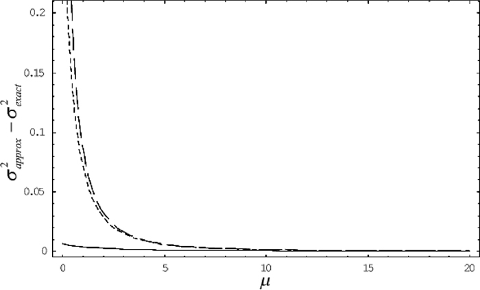View Details

Fig. 3 The difference between the approximate value of squared SLD and the exact one when the recombination rate c = 0.01 (dashed line), c = 1 (dotted line), c = 100 (line) along the mutation rate μ. Each c and μ is measured in units of 2N generations.

DISCUSSION

In this study I have developed an approximate formula for the simultaneous distribution of allele frequencies and linkage disequilibrium in terms of 2-locus 2-allele model with mutual mutations by using the small asymptotic disturbance theory. We confirmed that this approximate formula works well even at stationary state if the mutation rates are high. Furthermore, if the linkage is loose, namely if the recombination rate is high, the accuracy of the approximation increases.

The small asymptotic disturbance theory has a wide range of generalities.

Using this theory, we can readily expand the present 2-locus 2-allele model to the 2-locus multi-allelic one, though the complexity of calculation increases a little. We are also able to apply this formula to the Ancestral Recombination Graph (ARG) under proper conditions such as high mutation rate. Recently Mano (2009) derived the duality between the 2-locus diffusion process and the ARG when the process has no mutation. According to him, there is the following relationship between the process and the ARG;

where x_1t = p_tq_t + D_t and x₁₀ = p₀q₀ + D₀, namely the frequency of the haplotype A₁B₁. Each z_1t, z_2t, z_3t, represents the stochastic process of the number of lineage of haplotypes A₁ _, _ B₁, A₁B₁ respectively, where A₁ _ means the haplotype with allele A₁ at locus A and unspecified alleles at locus B, _ B₁ means the haplotype with allele B₁ at locus B and unspecified alleles at locus A. l, m, n are initial values of z_1t, z_2t, z_3t, respectively. This relationship will still hold when there exist mutations, if the mutation rates are the same in each locus. Hence under high and equal mutation rates, we can approximately calculate the relation

for example.

On the other hand, under improper situations such as low mutation rates, the approximate formula does not work well, and it is not possible to express the situation near boundaries of frequencies and around the origin of LD as have seen in the comparison with the simulation. Hence we have to design another way in order to treat the behavior near these singularities. Voronka and Keller (1975) obtained an asymptotic expression of the transient distribution of 1-locus 2-allele model with arbitrary selection pressure using the another method which is developed in the theory of wave propagation. As well as the small disturbance asymptotic theory, however, this method has a limitation in treating near boundaries, so they expressed the behavior near boundaries by using the boundary layer analysis. And this analysis is also able to be applied to internal boundary layer, namely around the origin. Thus we may be able to express the situation of singularities with boundary layer analysis in the present case, though the amount of computation increases largely.

I would like to express my deepest gratitude to my adviser Professor Fumio Tajima for support and encouragement throughout this study. I also appreciate Dr. Takahasi, K. R. and two anonymous reviewers for valuable comments and support.

APPENDIX

The concrete expression of the elements of (19) are calculated with the following form;

Then we obtain