RNA design using simulated SHAPE data

ABSTRACT

It has long been established that in addition to being involved in protein translation, RNA plays essential roles in numerous other cellular processes, including gene regulation and DNA replication. Such roles are known to be dictated by higher-order structures of RNA molecules. It is therefore of prime importance to find an RNA sequence that can fold to acquire a particular function that is desirable for use in pharmaceuticals and basic research. The challenge of finding an RNA sequence for a given structure is known as the RNA design problem. Although there are several algorithms to solve this problem, they mainly consider hard constraints, such as minimum free energy, to evaluate the predicted sequences. Recently, SHAPE data has emerged as a new soft constraint for RNA secondary structure prediction. To take advantage of this new experimental constraint, we report here a new method for accurate design of RNA sequences based on their secondary structures using SHAPE data as pseudo-free energy. We then compare our algorithm with four others: INFO-RNA, ERD, MODENA and RNAifold 2.0. Our algorithm precisely predicts 26 out of 29 new sequences for the structures extracted from the Rfam dataset, while the other four algorithms predict no more than 22 out of 29. The proposed algorithm is comparable to the above algorithms on RNA-SSD datasets, where they can predict up to 33 appropriate sequences for RNA secondary structures out of 34.

INTRODUCTION

Non-coding RNAs participate in various biological processes essential for cell survival, such as gene regulation and DNA replication (Storz and Gottesman, 2006). The function of these RNAs is dictated by their tertiary structures. Therefore, understanding the mutual relation between RNA structure and sequence sheds light on the biological role of RNAs. In fact, generating artificial RNA sequences folded to a desired RNA structure, RNA design (RD), is of known importance in drug design (Lagoja and Herdewijn, 2007).

In the last two decades, many algorithms and computational methods have been proposed for solving the RD problem (Churkin et al., 2017). For each given RNA secondary structure, RNAinverse (Hofacker et al., 1994) in the Vienna package (Lorenz et al., 2011) generates a sequence based on local search. INFO-RNA (Busch and Backofen, 2006) includes two main steps for designing an RNA sequence. First, a dynamic programming algorithm is employed to generate initial sequences, and then a stochastic local search is applied on the sequences. In the second step, neighbor sequences are evaluated based on distance minimization score. MODENA (Taneda, 2011) applies a multi-objective genetic algorithm in which a set of weak Pareto optimal sequences is generated based on the combination of structural stability and similarity scores. Frnakenstein (Lyngsø et al., 2012) uses a genetic algorithm based on multiple structural constraints. GGI-Fold (Ganjtabesh et al., 2013) also uses a multi-objective genetic algorithm to design sub-sequences for sub-structures derived from the target structure. The Gibbs sampling method is then applied to improve each sub-sequence. Finally, the sub-sequences are combined to design a sequence corresponding to the target structure. ERD (Esmaili-Taheri et al., 2014) uses an existing database of sequences (namely, STRAND [http://www.rnasoft.ca/strand/]) to design RNAs. In this algorithm, the target structure is divided into sub-structures such that each of them contains one multi-loop. A sub-sequence is then extracted from the database for each sub-structure. Finally, an evolutionary algorithm is employed to improve the combined sub-sequences folded to the target structure. RNAifold (Garcia-Martin et al., 2013, 2015) applies constraint programming and large neighborhood search algorithms for solving the RD problem.

In addition to the aforementioned RD algorithms using hard constraints, soft constraint-based methods have emerged to enhance the design process. AntaRNA employs both IUPAC format sequence and GC-content constraints to find the best sequence for a given structure using ant colony optimization (Kleinkauf et al., 2015). IncaRNAfbinv (Retwitzer et al., 2016) merges incaRNAtion (Reinharz et al., 2013) with RNAfbinv (Weinbrand et al., 2013) to solve the RD problem based on biologically meaningful constraints. RNAexinv (Avihoo et al., 2011) predicts a sequence for a given structure from shape representation and physical attributes.

In all of these methods, an RNA secondary structure prediction (RSSP) algorithm is applied to predict the structures of the designed sequences. Therefore, the quality of the final results is highly dependent on the RSSP algorithm. These approaches mainly apply hard constraints, such as minimum free energy (MFE), to evaluate RSSP. However, the results of these methods show that MFE cannot correctly predict some RNA secondary structures. Recently, the accuracy of RSSP has been improved by adding experimental SHAPE (selective 2’-hydroxyl acylation analyzed by primer extension) data (Wilkinson et al., 2006) to the free energy function as a soft constraint. SHAPE data correlate reactivity with flexibility of RNA nucleotides to predict the secondary structure (Low and Weeks, 2010). Although some algorithms, such as RNAstructure (Reuter and Mathews, 2010), GTfold (Mathuriya et al., 2009) and RNAsc (Zarringhalam et al., 2012), use SHAPE data as pseudo-free energy to increase the accuracy of RSSP, these data have never been employed to solve the RD problem. The reason is that obtaining the data experimentally itself requires RNA sequence, while the sequence is unknown in the RD problem. Thus, using SHAPE data in the RD algorithms remains a challenge. In this regard, a SHAPE data simulator could help the RD algorithms in designing more accurate sequences. Sükösd and colleagues presented a statistical model to simulate these data using three probability distribution functions for unpaired, stacked and helix-end nucleotide pairs (Sükösd et al., 2013).

In this paper, we show how to use simulated SHAPE data for RNA design. In this respect, a harmony search algorithm is presented to accurately predict RNA sequences folded to the target structure based on MFE and simulated SHAPE data as pseudo-free energy. For simulating SHAPE data, we use an extended version of the Sükösd simulator to provide a better solution for the RD problem.

We perform our algorithm on 29 RNA structures extracted from the database Rfam, known as a standard benchmark (Taneda, 2011), and 34 RNA structures from the RNA-SSD dataset (Andronescu et al., 2004). We compare our algorithm with four well-known algorithms, INFO-RNA (Busch and Backofen, 2006), ERD (Esmaili-Taheri et al., 2014), MODENA (Taneda, 2011) and RNAifold 2.0 (Garcia-Martin et al., 2015), on these datasets. Our algorithm precisely predicts 26 new sequences for the extracted structures from the Rfam dataset while the other algorithms predict 22 out of 29. The proposed algorithm is comparable to those algorithms on the RNA-SSD dataset, where they can predict 33 appropriate sequences for RNA secondary structures out of 34.

MATERIALS AND METHODS

In this section, some definitions and notations are explained to facilitate understanding of the proposed method. An RNA sequence is defined as follows:   

$$R=r_1{r}_2\dots r_n,\left|R\right|=n,r_i\in \left\{A,C,G,U\right\},1\le i\le n,$$

where A, C, G and U stand for adenine, cytosine, guanine and uracil, respectively. Each RNA secondary structure is formed by hydrogen bonds between complementary bases A = U, C ≡ G and G − U called base pairs. An assortment of unpaired bases and a set of consecutive base pairs are called a loop and a helix, respectively. Therefore, a secondary structure of RNA R can be defined as follows (Hofacker et al., 1994):   

$$S=s_1{s}_2\dots s_n,\left|S\right|=n,s_m\in \{\prime (\prime ,\prime )\prime ,\prime .\prime \},1\le m\le n,$$

where ′(′ and ′)′ represent a paired position and ‘.’ shows an unpaired position. A helix sub-structure (′h′) of S is displayed as a 4-tuple <′h′,i,j,k> where i < j and   

$$s_m=\{\begin{array}{c}\prime (\prime ,\mathrm{\hspace{0.17em} }\mathrm{\hspace{0.17em} }i\le m\le i+k-1,\\ \prime )\prime ,\mathrm{\hspace{0.17em} }\mathrm{\hspace{0.17em} }j\le m\le j+k-1.\end{array}$$

A loop sub-structure (′l′) of S is represented as a 4-tuple <′l′,i,i,k> where s_m = ′. ′ and i ≤ m ≤ i + k − 1.

Free energy of a given RNA secondary structure is computed as follows (Low and Weeks, 2010):   

$$\mathrm{\Delta }{G}_{FE}=\mathrm{\Sigma }\mathrm{\Delta }{G}_{helices}+\mathrm{\Sigma }\mathrm{\Delta }{G}_{loops},$$(1)

where ΔG_helices and ΔG_loops represent energy values of helices and loops of the secondary structure according to the laws of thermodynamics (Turner and Mathews, 2009). For each position i in a base pair, ΔG_i is calculated as pseudo-free energy using the following equation (Low and Weeks, 2010):   

$$\mathrm{\Delta }{G}_i=mln\left(SHAPE\mathrm{\hspace{0.17em} }reactivity\left(i\right)+1\right)+b,$$(2)

where SHAPE reactivity(i) is the SHAPE data of nucleotide i, and parameters m and b are set to 2.6 kcal/mol and −0.8 kcal/mol, respectively. Pseudo-free energy of the structure is computed as follows (Low and Weeks, 2010):   

$$\mathrm{\Delta }{G}_{SHAPE}=1\times \mathrm{\Sigma }\mathrm{\Delta }{G}_{start-end}+2\times \mathrm{\Sigma }\mathrm{\Delta }{G}_{interior},$$

where ΔG_start–end and ΔG_interior are calculated based on ΔG_i (Equation 2) for base pairs at the start, end (start-end) and interior of the helix. This pseudo-free energy is added to the free energy (Equation 1) according to the following formula for RNA secondary structure prediction (Low and Weeks, 2010):   

$$\mathrm{\Delta }{G}_{total}=\mathrm{\Delta }{G}_{FE}+\mathrm{\Delta }{G}_{SHAPE}.$$(3)

In the RD problem, our aim is to minimize ΔG_total (Equation 3) instead of ΔG_FE (Equation 1) for designing an RNA sequence that folds to a target structure.

The proposed algorithm for the RD problem

Harmony search is known as an appropriate evolutionary algorithm to solve multi-objective optimization problems (Yang, 2009). Since RNA design can be defined as a multi-objective problem (distance and free energy functions) (Taneda, 2011), it would be convenient to employ a harmony search algorithm in order to solve it.

A harmony search algorithm called HRDSSD is proposed for designing an RNA sequence using SHAPE data (http://bioinformatics.aut.ac.ir/HRDSSD/). The algorithm takes as input a target secondary structure S in order to predict the best sequence that can fold to the input structure. The details of random solutions for harmony memory, fitness function, a new harmonic and termination condition of the algorithm are described below.

Harmony memory

The numbers of harmonics, random RNA sequences, are produced as a harmony memory. To generate the kth harmonic, $R^k=r_1^k{r}_2^k\dots r_n^k,$ for target structure S = s₁s₂…s_n, a probabilistic approach is used. For each position i of R^k, a nucleotide is chosen with probability of P_t∈_{A,C,G,U} as follows:   

$$P_A\left(r_i^k=A\text{|}{s}_i\in \{\prime \text{(}\prime ,\prime .\prime \text{}}\right)=\frac{{\sum }_{j=1}^n\hspace{0.17em}{\chi }_{.}\left(s_j\right)}{n},$$

where   

$${\chi }_a\left(b\right)=\{\begin{array}{l}1\hspace{1em}\hspace{1em}a=b,\\ 0\hspace{1em}\hspace{1em}else.\end{array}$$

And   

$$P_{t\in \left\{C,G,U\right\}}=p\left(r_i^k=t\text{|}{s}_i\in \{\prime \text{(}\prime ,\prime .\prime \text{}}\right)=\frac{1-P_A}{3}.$$

The empty positions, $r_i^k$, are filled with the complements of their paired bases (A = U, C ≡ G and G − U).

Fitness function

For each pair of target secondary structure and RNA sequence in harmony memory, SHAPE data are simulated using the probability density functions (see sub-section 2.2). A secondary structure is computed for each designed sequence, based on minimizing ΔG_total (Equation 3) using GTfold (Mathuriya et al., 2009). The distance between predicted and target secondary structures is considered a fitness function.

Generating a new harmonic

To construct a new harmonic, the target structure S is decomposed to its sub-structures (helices, loops) and is added in a set Ω. Let a new harmonic be as follows:   

$$R^{new}=r_1^{new}{r}_2^{new}\dots r_n^{new},r_i^{new}=\text{N},1\le \text{i}\le \text{n},$$

where ‘N’ displays an unknown nucleotide in position i. A harmonic such as $R^H=r_1^H{r}_2^H\dots r_n^H$ is randomly selected from the harmony memory. The predicted structure of R^H is decomposed to sub-structures; and is added to the set Ω^H. Then, some 4-tuples, such as <p,i,j,k>∈Ω^H∩Ω, p∈{′l′, ′h′}, are randomly selected to set each $r_m^{new}$ to the nucleotide $r_m^H$ where, i ≤ m ≤ i + k − 1 and j ≤ m ≤ j + k − 1.

Random selection of a harmonic from the harmony memory is repeated to fill R^new with ‘A’s, ‘C’s, ‘G’s and ‘U’s until the generated random value is smaller than the harmony memory, considering rate. Finally, the unknown positions of R^new are randomly filled with ‘A’s, ‘C’s, ‘G’s or ‘U’s. The nucleotides corresponding to base pairs should be complementary.

Using this method, we generate 10 new harmonics. For each new harmonic, SHAPE data are simulated to compute ΔG_total (Equation 3) function using the probability functions (see sub-section 2.2). Then, these harmonics are sorted by the value of ΔG_total. One of the three first harmonics with the lowest fitness value (see sub-section 2.1.2) is replaced with the worst harmonic in the harmony memory, subject to the fitness value of this harmonic being better than the fitness value of the worst harmonic.

The algorithm terminates when the fitness value of the best harmonic is equal to 0, or the number of generations reaches |S|/4.

Simulating SHAPE data

As mentioned above, the HRDSSD algorithm generated some sequences for the target structure. For each sequence, the algorithm must compute the value of fitness function. A part of this function needs the SHAPE data for each nucleotide. Hence, we require a simulator to generate SHAPE data for each sequence and target structure. Although Sükösd et al. presented a statistical model to simulate these data for unpaired, stacked and helix-end pair bases (Sükösd et al., 2013), their model does not consider the type of nucleotides.

In this section, Sükösd’s simulator is extended to consider the type of nucleotides. The proposed stochastic method is constructed using the RNA sequences, native structures and experimental SHAPE data of 16S rRNA (1542 nt) and 23S rRNA (2904 nt) (K. M. Weeks, personal communication). We partitioned (into 12 clusters) the extracted SHAPE data from the following regions of these RNAs based on types of nucleotides:

(1) Unpaired region: represents a loop of RNA.

(2) Stacked region: shows consecutive base pairs except start and end of the helix.

(3) Helix-end region: indicates base pairs at the start and end of a helix.

For each cluster, a probability density function is generated by Easyfit 5.5 software (http://www.mathwaves.com). We employed this software because the size of each cluster (see Table 1) is not too large and it has been shown that the software is accurate for small sets (Disfani et al., 2012).

Table 1. Frequency of various nucleotides in unpaired, stacked and helix-end regions

	A	C	G	U
Unpaired	769	208	421	366
Stacked	236	534	600	387
Helix-end	78	196	302	90

Figures 1, 2, 3 display twelve probability density functions for estimating SHAPE data based on various nucleotides in different regions.

Fig. 1.

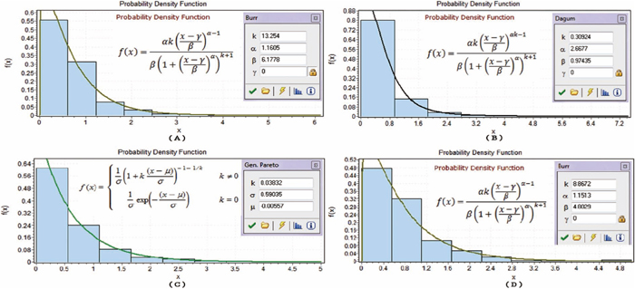
Probability density functions in unpaired regions. (A)–(D) show the probability density functions in the unpaired regions on nucleotides A, C, G and U, respectively.

Fig. 2.

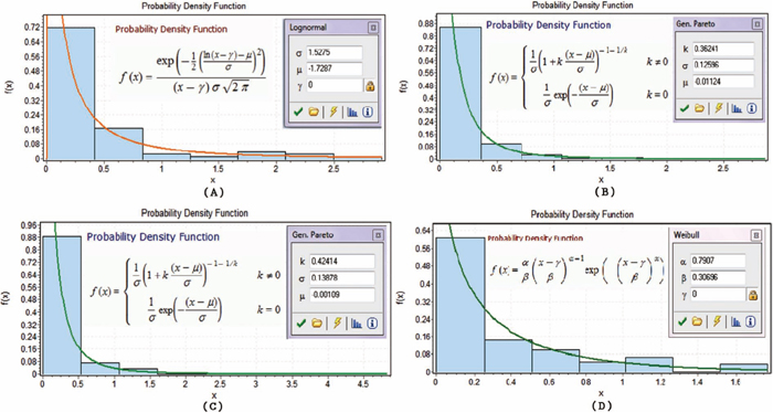
Probability density functions in stack regions. (A)–(D) show the probability density functions in the stack regions on nucleotides A, C, G and U, respectively.

Fig. 3.

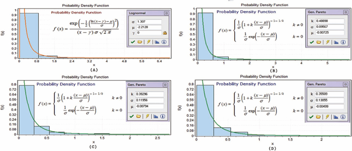
Probability density functions in helix-end regions. (A)–(D) show the probability density functions in the helix-end regions on nucleotides A, C, G and U, respectively.

RESUTS

In this section, we evaluate our algorithm, HRDSSD, on 29 RNAs extracted from the Rfam database, called dataset A (Taneda, 2011), and also datasets B and C obtained from RNA-SSD containing 24 and 10 RNAs, respectively (Andronescu et al., 2004). In this study, the HRDSSD algorithm is run on a machine with Intel(R) Core(TM) i5-2450M CPU 2.50 GHz and 4 GB RAM. We constrained the running time of the proposed algorithm to 10 minutes (Garcia-Martin et al., 2015) in each execution.

We compared three different versions of the proposed algorithm, our model (HRDSSD), the Sükösd model (HRDSSD-suko) and one without using SHAPE data (HRDWSD), to show that the simulated SHAPE data can improve the algorithm. HRDSSD is then compared to four well-known algorithms, ERD (Esmaili-Taheri et al., 2014), RNAifold 2.0 (Garcia-Martin et al., 2015), MODENA (Taneda, 2011) and INFO-RNA (Busch and Backofen, 2006).

Comparison of three different versions of the proposed algorithm

In this sub-section, we show the impact of the Sükösd model (three probability density functions (Sükösd et al., 2013)) and our model (twelve probability density functions) to design RNA sequences. Thus, we made a new version of HRDSSD called HRDSSD-suko by replacing the Sükösd model with our model to simulate SHAPE data. In addition, another version named HRDWSD is constructed by replacing ΔG_total (Equation 3) with ΔG_FE (Equation 1) to represent the effectiveness of simulated SHAPE data on the RD problem.

Table 2 shows the average time (Avg Time) and the number of RNA sequences designed accurately (NSDA) by the three versions of our algorithm on datasets A, B and C after 50 runs. The number of RNA sequences that are accurately designed by HRDSSD is higher than the number attained by the other algorithms. The results show that considering the type of nucleotides is important in SHAPE data simulation. The average time of HRSWSD is lower than the other methods because there is no extra computation for simulating SHAPE data.

Table 2. Comparison of HRDSSD, HRDSSD-suko and HRDWSD on datasets A, B and C (50 runs per structure, time limit set to 10 minutes)

	dataset A (29 structures)		dataset B (24 structures)		dataset C (10 structures)
Algorithm name	Avg Time	NSDA	Avg Time	NSDA	Avg Time	NSDA
HRDSSD	413.23	26	3868.72	24	35.74	9
HRDSSD- suko	338.24	25	4812.93	23	185.2	9
HRDWSD	71.70	24	1085.75	24	9.28	8

The details of our results for each RNA molecule in datasets A, B and C can be seen in columns 3–8 of Tables 5, 6, 7. The first and second columns of these tables show the name and length of the RNAs. The success count (SC) for each approach specifies the number of successful executions out of a total of 50 executions (10 minutes for each execution). The running time of each algorithm is the average time of successful runs in less than 10 minutes. If there is no successful run, the computational time is denoted by ‘–’.

Table 5. Comparison of HRDSSD and the other methods on dataset A (50 runs per structure, time limit set to 10 minutes)

Rfam AC	length	HRDSSD		HRDSSD-suko		HRDWSD		ERD		MODENA		INFO-RNA		RNAifold 2.0
		SC	time	SC	time	SC	time	SC	time	SC	Time	SC	time	SC	time
RF00001	117	50	1.94	50	10.12	50	2.18	50	0.92	28	0.79	49	0.15	27	8.52
RF00002	151	50	1.12	50	4.14	50	1.64	49	2.98	13	2.00	0	–	3	60.03
RF00003	161	50	2.00	50	8.20	23	17.00	41	5.94	11	2.18	0	–	0	–
RF00004	193	50	0.94	50	2.66	50	0.58	50	2.51	48	0.77	19	2.73	46	0.35
RF00005	74	50	0.28	50	0.66	50	0.30	50	0.03	35	0.37	49	0.04	47	0.08
RF00006	89	50	0.38	50	0.96	50	0.44	50	0.17	44	0.34	40	0.06	50	0.10
RF00007	154	50	0.86	50	2.96	50	0.82	50	0.71	48	0.58	42	0.30	44	0.40
RF00008	54	50	0.22	50	0.60	50	0.24	50	0.01	46	0.24	50	0.00	50	0.06
RF00009	348	50	9.50	50	32.04	49	11.73	49	22.52	39	3.13	0	–	8	1.27
RF00010	357	0	–	0	–	0	–	0	–	0	–	0	–	0	–
RF00011	382	1	282.00	0	–	0	–	0	–	0	–	0	–	0	–
RF00012	215	50	1.02	50	3.50	50	0.82	50	1.52	47	0.96	3	23.24	50	0.41
RF00013	185	50	0.96	50	3.20	50	0.70	50	1.42	38	1.13	13	2.00	50	0.42
RF00014	87	50	0.26	50	0.80	50	0.26	50	0.04	40	0.40	50	0.02	50	0.12
RF00015	140	50	0.54	50	2.08	50	0.58	50	0.86	44	0.57	19	1.74	47	0.33
RF00016	129	0	–	0	–	0	–	0	–	0	–	0	–	0	–
RF00017	301	50	2.18	50	10.00	50	1.14	50	2.13	42	2.76	48	0.80	48	2.49
RF00018	360	50	10.12	50	42.46	50	7.04	0	–	0	–	0	–	0	–
RF00019	83	50	0.36	50	1.04	50	0.30	50	0.09	46	0.33	47	0.03	50	0.10
RF00020	119	50	0.54	50	1.80	0	–	0	–	0	–	0	–	0	–
RF00021	118	50	0.28	50	0.74	50	0.26	50	0.13	40	0.63	50	0.09	50	0.58
RF00022	148	50	0.50	50	1.44	50	0.48	50	1.02	44	0.68	8	1.05	42	0.21
RF00024	451	0	–	0	–	0	–	0	–	0	–	0	–	0	–
RF00025	210	50	1.06	50	3.50	50	0.68	50	3.36	45	0.87	1	0.93	50	0.33
RF00026	102	50	0.24	50	0.54	50	0.22	50	0.02	45	0.36	2	3.11	50	0.06
RF00027	79	50	0.28	50	0.64	50	0.28	50	0.03	49	0.35	50	0.04	50	0.21
RF00028	344	46	87.33	41	174.54	45	17.67	50	26.42	0	–	0	–	1	1.54
RF00029	73	50	0.34	50	0.88	50	0.40	50	0.06	39	0.28	3	0.01	50	0.08
RF00030	340	50	7.98	50	28.74	50	5.94	0	–	44	2.34	0	–	26	5.55
sum		1247	413.23	1241	338.24	1167	71.70	1089	72.88	875	22.05	543	36.32	889	83.25

Table 6. Comparison of HRDSSD and the other methods on RNA-SSD dataset B (50 runs per structure, time limit set to 10 minutes)

id rnassd1	length	HRDSSD		HRDSSD-suko		HRDWSD		ERD		MODENA		INFO-RNA		RNAifold2.0
		SC	time	SC	time	SC	Time	SC	time	SC	time	SC	time	SC	time
AB015827	857	50	152.66	49	223.02	50	13.32	50	7.15	45	20.64	37	11.68	39	40.66
AF029195	1054	50	525.42	48	354.40	50	29.66	50	11.58	0	–	47	32.67	43	2.15
AF056938	1399	50	841.30	38	1738.50	50	30.08	50	43.85	0	–	43	112.64	0	–
AF096836	647	50	22.76	49	118.06	50	4.48	50	4.32	0	–	43	3.40	35	16.13
AF106618	351	50	5.18	50	24.62	50	1.54	50	1.84	41	3.56	47	0.58	49	4.58
AF107506	338	50	3.76	50	24.60	50	1.78	50	2.38	39	3.59	44	2.04	1	2.19
AF141485	474	50	10.64	50	78.30	50	3.32	50	3.42	45	5.93	33	4.61	0	–
AJ011149	377	50	12.38	50	41.38	48	6.85	50	1.43	0	–	37	1.72	22	2.90
AJ130779	507	50	13.58	49	109.71	50	3.98	50	2.41	47	6.19	49	1.72	19	9.87
AJ132572	781	50	103.62	38	312.26	50	9.98	50	7.12	0	–	42	12.90	22	18.87
AJ133622	1297	1	599.00	34	62.06	26	176.23	50	18.79	0	–	49	233.92	45	289.25
AJ236455	752	6	314.17	2	341.50	11	136.18	50	18.22	0	–	5	255.65	0	–
D38777	859	50	162.08	20	342.20	50	17.08	50	14.14	0	–	42	164.69	0	–
L11935	265	50	1.92	50	7.04	50	0.80	50	0.78	49	1.51	49	0.81	50	1.21
L77117	1476	2	298.50	4	238.00	4	238.00	50	23.63	0	–	50	55.28	0	–
LIU92530	290	7	90.57	4	191.00	15	62.73	50	1.02	0	–	22	1.26	43	4.08
S70838	390	46	50.57	46	89.80	48	7.38	50	2.99	0	–	46	2.96	49	18.11
U63350	419	50	5.14	50	26.06	50	1.76	50	1.54	49	4.14	48	3.49	44	4.73
U81771	492	50	7.80	50	57.76	50	2.28	50	1.99	0	–	46	2.71	0	–
U84629	300	48	19.46	46	53.48	49	4.55	50	0.97	5	19.40	40	2.40	50	2.43
X61771	660	49	86.18	36	383.28	49	92.47	50	13.19	0	–	17	17.09	0	–
X81949	1201	18	340.50	39	82.00	47	206.45	50	17.76	0	–	48	128.07	31	19.23
X99676	1443	2	544.50	0	–	4	40.50	50	31.17	0	–	46	220.37	0	–
Z83250	261	50	6.10	50	3.70	50	1.72	50	0.68	35	2.20	50	0.74	45	1.85
sum		929	3868.72	902	4812.93	1001	1085.75	1200	232.35	355	67.17	980	1273.41	587	438.22

Table 7. Comparison of HRDSSD and the other methods on RNA-SSD dataset C (50 runs per structure, time limit set to 10 minutes)

id SSD2	length	HRDSSD		HRDSSD-suko		HRDWSD		ERD		MODENA		INFO-RNA		RNAifold2.0
		SC	time	SC	time	SC	time	SC	time	SC	Time	SC	time	SC	time
1	65	50	0.2	50	0.72	50	0.28	50	0.04	39	0.31	50	0.02	50	0.10
2	79	50	0.26	50	0.7	50	0.3	50	0.03	46	0.35	50	0.01	50	0.09
3	122	50	1.7	50	5.44	50	0.96	50	0.29	6	3.33	50	0.06	50	0.18
4	166	50	0.72	50	2.26	50	0.44	50	0.34	50	0.86	50	0.10	50	0.53
5	180	50	5.12	50	40.58	0	–	8	9.28	0	–	0	–	0	–
6	314	50	2.26	50	9.24	50	1.26	50	4.83	49	1.92	11	10.95	11	1.51
7	340	50	4.12	50	12.84	50	1.56	50	3.19	45	2.64	14	23.02	24	2.29
8	372	50	5.1	50	16.34	50	1.66	50	13.94	46	3.02	4	31.17	25	2.19
9	376	0	–	0	–	0	–	0	–	0	–	0	–	0	–
10	583	50	16.26	50	97.08	50	2.82	50	4.39	45	9.24	43	8.00	12	9.68
Sum		450	35.74	450	185.2	400	9.28	408	36.32	326	21.68	272	73.34	272	16.58

Next, we show that the 3D structures of the RNA sequences designed using SHAPE data are more similar to the native structures. To do this, we select the 3D structures of six RNAs from PDB whose secondary structures are pseudoknot-free (see Table 3). The 3D structures of these RNAs are then converted to secondary structures by DSSR software (Lu et al., 2015).

Table 3. The RNA dataset extracted from PDB

PDB id	Length	PDB id	Length
1a51	41	1kxk	70
1cq5	43	1jxr	46
1kqs chain 9	122	3JQ4 chain B	118

Next, each structure is given as an input to HRDSSD, HRDSSD-suko and HRDWSD algorithms ten times. The output sequences are given to RNAcomposer (Popenda et al., 2012) to predict the 3D structures. Finally, these structures are aligned to the PDB structures by the Rclick server (Nguyen and Verma, 2015). Table 4 shows the average overlap between the predicted 3D structure of each designed RNA sequence and its real 3D structure.

Table 4. Average structure overlap between the predicted and real 3D structures

PDB id	HRDSSD	HRDSSD-suko	HRDWSD
1a51	56.1	19.76	53.90
1cq5	19.77	23.25	21.86
1kqs chain 9	18.36	18.44	18.28
1kxk	19.29	18.71	14.86
1jxr	21.30	20.22	20
3JQ4 chain B	35.34	32.97	32.46
Average	28.36	22.22	26.89

The average structure overlap represented by HRDSSD shows that this method may design RNA sequences more similar to those in nature.

Comparison of HRDSSD with four well-known algorithms

Columns 9 to 16 of Tables 5, 6, 7 present the results of the INFO-RNA, RNAifold 2.0, MODENA and ERD algorithms on datasets A, B and C. As shown, the proposed approach precisely predicts 26 new sequences for the extracted structures from dataset A, while the other four methods can design at most 22 accurate RNA sequences. HRDSSD is comparable to the other methods on datasets B and C where they can predict 33 accurate sequences for RNA secondary structures out of 34.

As shown in Tables 5, 6, 7, the running time of our algorithm (HSDSSD) is not as fast as the other algorithms, because most of these algorithms employ the Vienna RNA package (Lorenz et al., 2011) for predicting the secondary structure of designed sequences. Although GTfold is the fastest software that uses SHAPE data, the Vienna RNA package, which uses only the free energy function, is faster. In other words, applying SHAPE data in any RNA secondary structure prediction algorithm would consume more time.

CONCLUSION

In this paper, we developed a model to simulate SHAPE data taking into account different types of nucleotides in each region of an RNA. In this model, twelve probability density functions were fitted for various nucleotides in loops, stacked and helix-end pair regions. A harmony search algorithm called HDRSSD was then employed to design an RNA sequence for the given secondary structure by simulated SHAPE data. The proposed algorithm, HDRSSD, predicted more accurate RNA sequences than the other algorithms on the databases Rfam and RNA-SSD. The results showed that SHAPE data not only improve RNA secondary structure prediction, but also improve the RD algorithms.

ACKNOWLEDGMENTS

Special thanks to Ms. Parisa Hosseinzadeh and Bita Pourmohsenin for their help in editing the article.

REFERENCES

•  Andronescu,  M.,  Fejes,  A. P.,  Hutter,  F.,  Hoos,  H. H., and  Condon,  A. (2004) A new algorithm for RNA secondary structure design. J. Mol. Biol. 336, 607–624.
•  Avihoo,  A.,  Churkin,  A., and  Barash,  D. (2011) RNAexinv: An extended inverse RNA folding from shape and physical attributes to sequences. BMC Bioinformatics 12, 319.
•  Busch,  A., and  Backofen,  R. (2006) INFO-RNA—a fast approach to inverse RNA folding. Bioinformatics 22, 1823–1831.
•  Churkin,  A.,  Retwitzer,  M. D.,  Reinharz,  V.,  Ponty,  Y.,  Waldispühl,  J., and  Barash,  D. (2017) Design of RNAs: comparing programs for inverse RNA folding. Brief. Bioinform.18 1–9.
•  Disfani,  F. M.,  Hsu,  W. L.,  Mizianty,  M. J.,  Oldfield,  C. J.,  Xue,  B.,  Dunker,  A. K.,  Uversky,  V. N., and  Kurgan,  L. (2012) MoRFpred, a computational tool for sequence-based prediction and characterization of short disorder-to-order transitioning binding regions in proteins. Bioinformatics 28, i75–i83.
•  Esmaili-Taheri,  A.,  Ganjtabesh,  M., and  Mohammad-Noori,  M. (2014) Evolutionary solution for the RNA design problem. Bioinformatics 30, 1250–1258.
•  Ganjtabesh,  M.,  Zare-Mirakabad,  F., and  Nowzari-Dalini,  A. (2013) Inverse RNA folding solution based on multi-objective genetic algorithm and Gibbs sampling method. EXCLI J. 12, 546–555.
•  Garcia-Martin,  J. A.,  Clote,  P., and  Dotu,  I. (2013) RNAiFOLD: a constraint programming algorithm for RNA inverse folding and molecular design. J. Bioinform. Comput. Biol. 11, 1350001.
•  Garcia-Martin,  J. A.,  Dotu,  I., and  Clote,  P. (2015) RNAiFold 2.0: a web server and software to design custom and Rfam-based RNA molecules. Nucleic Acids Res, 43, W513–W521.
•  Hofacker,  I. L.,  Fontana,  W.,  Stadler,  P. F.,  Bonhoeffer,  L. S.,  Tacker,  M., and  Schuster,  P. (1994) Fast folding and comparison of RNA secondary structures. Monatsh. Chem. 125, 167–188.
•  Kleinkauf,  R.,  Mann,  M., and  Backofen,  R. (2015) antaRNA: ant colony-based RNA sequence design. Bioinformatics 31, 3114–3121.
•  Lagoja,  I. M., and  Herdewijn,  P. (2007) Use of RNA in drug design. Expert Opin. Drug Discov. 2, 889–903.
•  Lorenz,  R.,  Bernhart,  S. H.,  Höner zu Siederdissen,  C.,  Tafer,  H.,  Flamm,  C.,  Stadler,  P. F., and  Hofacker,  I. L. (2011) ViennaRNA Package 2.0. Algorithms For Mol. Biol. 6, 26.
•  Low,  J. T., and  Weeks,  K. M. (2010) SHAPE-directed RNA secondary structure prediction. Methods 52, 150–158.
•  Lu,  X.-J.,  Bussemaker,  H. J., and  Olson,  W. K. (2015) DSSR: an integrated software tool for dissecting the spatial structure of RNA. Nucleic Acids Res. 43, e142.
•  Lyngsø,  R. B.,  Anderson,  J. W. J.,  Sizikova,  E.,  Badugu,  A.,  Hyland,  T., and  Hein,  J. (2012) Frnakenstein: multiple target inverse RNA folding. BMC Bioinformatics 13, 260.
•  Mathuriya,  A.,  Bader,  D. A.,  Heitsch,  C. E., and  Harvey,  S. C. (2009) GTfold: a scalable multicore code for RNA secondary structure prediction. In Proceedings of the 2009 ACM symposium on Applied Computing, pp. 981–988. ACM, New York.
•  Nguyen,  M. N., and  Verma,  C. (2015) Rclick: a web server for comparison of RNA 3D structures. Bioinformatics, 31, 966–968.
•  Popenda,  M.,  Szachniuk,  M.,  Antczak,  M.,  Purzycka,  K. J.,  Lukasiak,  P.,  Bartol,  N.,  Blazewicz,  J., and  Adamiak,  R. W. (2012) Automated 3D structure composition for large RNAs. Nucleic Acids Res. 40, e112.
•  Reinharz,  V.,  Ponty,  Y., and  Waldispühl,  J. (2013) A weighted sampling algorithm for the design of RNA sequences with targeted secondary structure and nucleotide distribution. Bioinformatics 29, i308–i315.
•  Retwitzer,  M. D.,  Reinharz,  V.,  Ponty,  Y.,  Waldispühl,  J., and  Barash,  D. (2016) incaRNAfbinv: a web server for the fragment-based design of RNA sequences. Nucleic Acids Res. 44, W308–W314.
•  Reuter,  J. S., and  Mathews,  D. H. (2010) RNAstructure: software for RNA secondary structure prediction and analysis. BMC bioinformatics 11, 129.
•  Storz,  G., and  Gottesman,  S. (2006) 20 Versatile Roles of Small RNA Regulators in Bacteria. Cold Spring Harbor Monograph Archive 43, 567–594.
•  Sükösd,  Z.,  Swenson,  M. S.,  Kjems,  J., and  Heitsch,  C. E. (2013) Evaluating the accuracy of SHAPE-directed RNA secondary structure predictions. Nucleic Acids Res. 41, 2807–2816.
•  Taneda,  A. (2011) MODENA: a multi-objective RNA inverse folding. Adv. Appl. Bioinform. Chem. 4, 1–12.
•  Turner,  D. H., and  Mathews,  D. H. (2009) NNDB: the nearest neighbor parameter database for predicting stability of nucleic acid secondary structure. Nucleic Acids Res. 38, D280–D282.
•  Weinbrand,  L.,  Avihoo,  A., and  Barash,  D. (2013) RNAfbinv: an interactive Java application for fragment-based design of RNA sequences. Bioinformatics 29, 2938–2940.
•  Wilkinson,  K. A.,  Merino,  E. J., and  Weeks,  K. M. (2006) Selective 2’-hydroxyl acylation analyzed by primer extension (SHAPE): quantitative RNA structure analysis at single nucleotide resolution. Nat. Protoc. 1, 1610–1616.
•  Yang,  X.-S. (2009) Harmony search as a metaheuristic algorithm. In Music-Inspired Harmony Search Algorithm. (ed.: Geem, Z. W.), pp. 1–14. Springer, Heidelberg.
•  Zarringhalam,  K.,  Meyer,  M. M.,  Dotu,  I.,  Chuang,  J. H., and  Clote,  P. (2012) Integrating chemical footprinting data into RNA secondary structure prediction. PloS One 7, e45160.