Transient Fluid Flow during Steady Continuous Casting of Steel Slabs: Part I. Measurements and Modeling of Two-phase Flow

Abstract

Unstable mold flow could induce surface velocity and level fluctuations, and entrain slag, leading to surface defects during continuous casting of steel. Both argon gas injection and Electro-Magnetic Braking (EMBr) greatly affect transient mold flow and stability. Part I of this two-part article investigates transient flow of steel and argon in the nozzle and mold during nominally steady-state casting using both plant measurements and computational modeling. Nail board dipping measurements are employed to quantify transient surface level, surface velocity, flow direction, and slag depth. Transient flow in the nozzle and strand is modeled using Large Eddy Simulation (LES) coupled with the Lagrangian Discrete Phase Model (DPM) for argon gas injection. The surface level of the molten steel fluctuates due to sloshing and shows greater fluctuations near the nozzle. The slag level fluctuates with time according to the lifting force of the molten steel motion below. Surface flow shows a classic double roll pattern with transient cross-flow between the Inside Radius (IR) and the Outside Radius (OR), and varies with fluctuations up to ~50% of the average velocity magnitude. The LES results suggest that these transient phenomena at the surface are induced by up-and-down jet wobbling caused by transient swirl in the slide-gate nozzle. The jet wobbling influences transient argon gas distribution and the location of jet impingement on the Narrow Face (NF), resulting in variations of surface level and velocity. A power-spectrum analysis of the predicted jet velocity revealed strong peaks at several characteristic frequencies from 0.5–2 Hz (0.5–2 sec).

1. Introduction

Continuous casting is used to manufacture over 95% of steel in the world¹⁾ and many defects in this process are related to transient fluid flow in the mold region. Thus, small improvements to understanding transient flow phenomena and its effect on steel product quality can lead to large savings. Variations of surface level and surface velocity in the mold of the continuous caster are well known as the most important factors responsible for the defects related with fluid flow phenomena. Severe surface level fluctuations can entrap slag into the molten steel.^2,3) Abnormal high surface velocity and velocity variations, leading to asymmetric surface flow, vortex formation,^4,5) and instability at the interface between the molten steel and slag,^6,7,8) could entrain slag into the molten steel, causing both surface and internal defects in the steel product. On the other hand, abnormal slow surface flow could result in low and non-uniform surface temperature, inducing insufficient slag melting and infiltration, meniscus freezing, hook formation,^9,10) and surface defects related to initial solidification problems. Argon gas is injected to prevent nozzle clogging in continuous steel casting, but may cause complexity and instability of transient flow pattern. Applying a magnetic field induces Electro-Magnetic Braking (EMBr) forces which also affect transient mold flow and stability. It is important to understand the effects of argon gas and EMBr on transient fluid flow to prevent defects during the continuous casting. This two-part article investigates the effects of argon gas (Part I) and EMBr (Part II) on transient flow in the nozzle and mold, focusing on surface behavior.

Many researchers have investigated the effect of argon gas on time-averaged flow in the nozzle and mold.^{11,12,13,14,15,16,17,18,19,20,21)} However, there is less study on the effect of gas on transient flow.^{22,23,24,25,26)} Using a standard steady-state k–ε model, Bai and Thomas found that increasing argon gas volume fraction or bubble diameter bends the jet angle more upward and also increases turbulence.²²⁾ Using Large Eddy Simulation (LES) and water modeling, several studies observed long-term asymmetry and unbalanced transient flow in the lower rolls, causing bubbles to penetrate deeply.^23,24) Using nail-board dipping tests, Kunstreich et al.²⁵⁾ and Dauby²⁶⁾ found detrimental ranges of operating conditions including argon gas injection rates that caused unstable, complex flow, resulting in defects. Both transient computational model and plant measurements are needed to understand quantitatively transient flow and to find methods to prevent defects.

In Part I of this two-part article, transient flow of molten steel and argon gas during steady continuous casting of steel slabs is investigated by applying both plant measurements and computational modeling. Nail board dipping tests quantify transient and time–averaged surface level and surface velocity of molten steel. Thickness and level motion of the liquid mold flux (slag) are also investigated. Further insight into transient flow in the nozzle and mold is quantified by LES coupled with Lagrangian Discrete Phase Model (DPM) for argon gas injection. Power spectrum analysis of the predicted velocity history was performed to reveal the transient variations and characteristic frequencies.

2. Plant Experiments

Plant measurements were conducted on a conventional continuous steel slab continuous caster at POSCO Gwangyang Works #2-1 caster in 2008 and in 2010. Results from 2010 measurements are included here while Part 2 includes both trials. Processing conditions for the plant measurements are given with nozzle and mold dimensions in Table 1. Flow in this 250 × 1300 mm caster is through a standard bifurcated Submerged Entry Nozzle (SEN) with rectangular ports, controlled by a slide-gate system with middle plate movement between Outside Radius (OR) and Inside Radius (IR) as shown in Fig. 1. During the measurements, argon gas of 9.2 SLPM was injected through the Upper Tundish Nozzle (UTN), and expanded to 33.0 LPM. The heated gas occupies 5.6% volume fraction, F_Ar, of the total volume flow rate of the molten steel, Q_s and the argon gas, Q_{Ar, 1827 K}, calculated as follows   

$${\text{F}}_{\text{Ar}}=\frac{{\text{Q}}_{\text{Ar, 1}\mathrm{\hspace{0.17em} }\text{827 K}}}{{\text{Q}}_{\text{s}}+{\text{Q}}_{\text{Ar, 1}\mathrm{\hspace{0.17em} }\text{827 K}}}\times \text{100}$$(1)

  

$${\text{Q}}_{\text{s}}={\text{W}}_{\text{mold}}\times {\text{T}}_{\text{mold}}\times {\text{U}}_{\text{casting}}$$(2)

where W_mold is mold width, T_mold mold thickness, and U_casting casting speed.   

$$\begin{array}{l}{\text{Q}}_{\text{Ar,1}\mathrm{\hspace{0.17em} }\text{827 K}}={\text{Q}}_{\text{Ar, 273 K}}\times \left(\frac{{\text{P}}_{\text{273 K}}}{{\text{P}}_{\text{1}\mathrm{\hspace{0.17em} }\text{827 K}}}\right)\times \left(\frac{\text{1}\mathrm{\hspace{0.17em} }\text{827 K}}{\text{273 K}}\right)\\ {\text{where P}}_{\text{1}\mathrm{\hspace{0.17em} }\text{827K}}={\text{P}}_{\text{s,tundish\_level}}+\rho \text{gh}-\frac{\text{1}}{\text{2}}\rho {\left({\text{U}}_{\text{s,UTN}}\right)}^{\text{2}}\end{array}$$(3)

where P_{s,tundish_level} is pressure at the tundish surface (1 atm), ρ is molten steel density, h is distance from tundish surface to the gas outlets, and U_s,UTN is the mean velocity of molten steel in the nozzle.

Table 1. Caster dimensions and process conditions.

Caster Dimensions
Nozzle bore diameter (inner/outer)	90 mm (at UTN top) to 80 mm (at bottom well) / 160 mm (at UTN top) to 140 mm (at SEN bottom)
Nozzle bottom well depth	19 mm
Nozzle port area	80 mm (width) × 85 mm (height)
Nozzle port angle	*2008: 52 to 35 down degree step angle at the top, 45 down degree angle at the bottom *2010: 35 down degree angle at both top and bottom
Mold thickness	250 mm
Mold width	1300 mm
Domain length	4648 mm (mold region: 3000 mm (below mold top))
Process Conditions
Steel flow rate	552.5 LPM (3.9 tonne/min)
Casting speed	1.70 m/min (28.3 mm/sec)
Argon gas flow rate & volume fraction	9.2 SLPM (1 atm, 273 K); 33.0 LPM (1.87 atm, 1827 K) & 5.6% (hot)
Submerged depth of nozzle	164 mm
Meniscus level below mold top	103 mm
EMBr current (both coils)	DC 300 A

Fig. 1.

(a) Schematic of slide-gate in steel slab continuous casting and (b) slide-gate middle plate on SEN. (Online version in color.)

Transient surface level and velocity in the mold were quantified via both eddy-current sensor measurements and nail board dipping tests. The mold water-box had a cavity that contained the static DC magnets for a double-ruler EMBr system by ABB. The applied field strength was measured without molten steel using a Gauss meter.

2.1. Eddy-current Senor Measurements

The eddy-current sensor detects the surface level, and sends the signal to a controller, which aims to maintain a constant average liquid level in the mold by moving the middle plate of the slide-gate to adjust the open area of the nozzle. This sensor was positioned over the “quarter point” located midway between the SEN and Narrow Face (NF). If the level drops slightly, the slide-gate opens to increase flow rate until the level returns to the set-point, located 103 mm below top of the mold. The sensor signal sent to the controller is filtered intentionally to remove the high frequency level variations, which cannot be controlled. Averages, standard deviations, and power spectra of the 1 sec moving time-average of the surface level signal in 2010 trial were calculated both with and without EMBr and are presented in Part II.

2.2. Nail Board Dipping Tests

Nail board dipping tests were conducted to quantify surface level, surface velocity, and their fluctuations for the trials in both 2008 and 2010. Nail board dipping tests are commonly used to investigate mold surface flow due to their convenience and efficiency.^{27,28,29,30,31)} In these trials, two rows of ten 5 mm-diameter, 290 mm-long STainless Steel (STS) nails, spaced 50 mm apart were attached to each wood board, together with 3 mm diameter aluminum nails, as shown in Fig. 2. The nail board with the STS and Al nails was immersed into the mold, centered between the IR and OR, and between the SEN and the NF on the opposite side from the eddy-current sensor. The nail board is supported above the oscillating mold on two bent rods to keep it stable and level without tilting. As molten steel flows around the nails, it is pushed up on the windward side, and down on the leeward side, so solidifies an angled lump around each nail. As shown in Fig. 3, after taking out the nails from the molten steel pool, these solidified steel lumps are used to reveal the liquid level profile and the velocity across the top of the mold. Surface velocity at the nail is estimated from the measured lump height difference h_lump (mm), and lump diameter ϕ_lump (mm), using the empirical equation developed by Liu et al.²⁹⁾ based on the data of computational modeling by Rietow et al.³⁰⁾   

$${\text{V}}_{\text{surface}}=\text{0}\text{.624}\cdot {\left({\varphi }_{\text{lump}}\right)}^{-0.696}\cdot {\left({\text{h}}_{\text{lump}}\right)}^{0.567}$$(4)

Fig. 2.

Photos of the nail board: (a) top view, (c) front view and schematics of the nail board: (b) top view, (d) NF view. (Online version in color.)

Fig. 3.

Nail board dipping method. (Online version in color.)

For each test, the nail board was dipped into the molten steel pool for ~3 sec with 1 minute time interval between tests. The slag layer thickness h_slag is estimated from the height difference between the steel lump and the melted-back aluminum nail.

2.3. Magnetic Field Measurements

The magnetic field applied by the double ruler EMBr was measured using a Gauss meter at 69 data points in the mold cavity without molten steel. On each of three vertical lines, located 0, 350, and 700 mm from the mold center, 23 positions are measured by lowering the Gauss meter downward in 50 mm increments from the mold top. The measurements were extrapolated to cover the entire nozzle and mold, and input to a standard k–ε model with EMBr, as discussed in detail in Part II.

3. Plant Measurement Results

Plant measurement results in this paper are from the 2010 trial (no EMBr) and are presented in Figs. 4, 5, 6, 7, 8 for surface level and velocity.

Fig. 4.

Transient variations of surface level profile by the nail board measurements. (Online version in color.)

Fig. 5.

(a)Time-averaged surface level and (b) surface level fluctuation by the nail board measurements. (Online version in color.)

Fig. 6.

Transient variations of surface flow pattern by the nail board measurements. (Online version in color.)

Fig. 7.

Averaged surface flow pattern by the nail board measurements. (Online version in color.)

Fig. 8.

(a) Time-averaged surface velocity and (b) surface velocity fluctuation by the nail board measurements. (Online version in color.)

3.1. Surface Level

The transient surface level profile of the interface between the molten steel and the slag layer in the mold was quantified during a 9-minute time interval via 10 nearly instantaneous snapshots using nail board dipping tests and are shown in Fig. 4. The time-average of these surface level shapes is shown in Fig. 5(a), and the surface level fluctuations are presented as the standard deviation of the snapshots in Fig. 5(b). These surface level profiles reveal evidence of transient low-frequency sloshing or waves between the SEN and the NF. Usually, surface level near the SEN and the NF is higher than at the quarter point, which is typical of surface behavior induced by a classic double roll pattern in the mold. With progressing time, the level profiles change, with the NF region higher at the same time the SEN region is lower, and vice versa. The magnitude of these rising and falling levels is up to 20 mm, (e.g. Fig. 4 frames 7 and 8). The sloshing period is shorter than 1 minute, and other fluctuations complicate the profiles, so it is not easy to see in Fig. 4 alone. Surface level fluctuations shown in Fig. 5(b) become more severe towards the SEN. In the quarter point region, surface level is the lowest and also exhibits the highest stability. Surface level fluctuations near the NF are intermediate. This is consistent with a slow sloshing mechanism, where the surface level pivots around the quarter point region.

The surface level of the steel-slag interface near the OR is usually slightly higher than near the IR. The level fluctuations near the OR were also slightly higher in the 2008 trial,³¹⁾ but not in the 2010 trial shown here in Fig. 5(b), so this trend is not consistent and needs further study with more data.

Slag level profiles, also shown in Figs. 4 and 5, show corresponding transient flow with sloshing, as influenced by the molten steel level motions. The slag surface level shape is similar to that of the steel. These results suggest that the slag level is simply lifted up and down by the molten steel motion. This contrasts with previous findings,³²⁾ where large differences in slag layer thickness were observed due to slag flow from the high NF region towards the SEN, which resulted in a thinner slag layer near the NF due to displacement. Perhaps there was insufficient time for slag flow due to gravity and displacement in the current study, or perhaps the effective slag viscosity was lower in the previous study, owing to foam formation from the higher argon flow.³³⁾ The relation of the surface level motion between the molten steel and the slag will be further discussed in detail in Part II.

3.2. Surface Velocity

Transient evolution of the surface flow pattern and velocity of the molten steel is visualized during the 9 minute period by snapshots taken 1 minute apart, and are shown in Fig. 6. Each surface flow pattern snapshot shows flow direction vectors as arrows with velocity magnitude represented by the length of each arrow. Most flow is towards the SEN, which is typical of a classic double-roll flow pattern in the mold. The profiles also show significant time variation and strong fluctuating cross-flow between the IR and OR. This surface cross-flow indicates variable asymmetric flow in the mold, likely related to the slide-gate movement between OR and IR, which induces swirl at the nozzle ports.³⁴⁾ Most surface flow is slightly biased from the OR towards the IR. This effect is clearly seen in the measurements of the row of nails near the OR. Surface flows measured near the IR show strong random variations towards either the IR or the OR. Surface flow very near the NF mostly goes towards the NF or the IR. This suggests a small region of recirculating flow in the top of the mold near the NF. Time-averaging of these surface flow patterns, given in Fig. 7 confirms the biased cross-flow towards the IR.

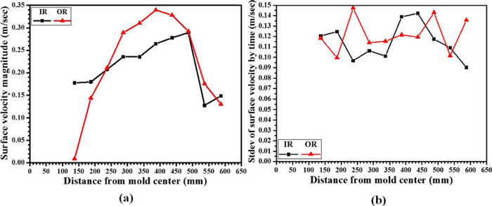
The velocity magnitudes across the mold are shown in Fig. 8(a), and their variations are given in Fig. 8(b). Higher surface velocities are found towards the quarter point, midway between the SEN and the NF, as typical for a double-roll flow pattern^13,17,35) The highest velocity is found closer to the OR. Surface velocity fluctuations are consistently very large ~0.12 m/sec across the entire mold width. These chaotic fluctuations are almost 50% of the average surface velocity magnitude for both the IR and the OR. This finding suggests that surface velocity fluctuations may be even more important than average surface velocity to understand surface flow phenomena related to defect formation.

4. Computational Models

Three-dimensional finite-volume computational models, including a standard k–ε model and LES coupled with a Lagrangian Discrete Phase Model (DPM) were applied to predict transient flow of molten steel and argon gas in the nozzle and mold. First, steady-state single-phase flow of molten steel was predicted with the standard k–ε model. Then, LES coupled with Lagrangian DPM was applied to calculate transient molten steel flow with argon gas, starting from the steady-state single-phase flow field. These models were implemented into the commercial package ANSYS FLUENT³⁹⁾ and are summarized below.

4.1. Single-phase (Molten Steel) Model of Steady Flow

A steady-state Reynolds Averaged Navier-Stokes (RANS) model using the standard k–ε model for turbulence was used to model single-phase flow. The continuity equation for mass conservation is given as   

$$\frac{\partial }{\partial {\text{x}}_{\text{i}}}\left(\rho {\overline{\text{u}}}_{\text{i}}\right)={\text{S}}_{\text{shell,}\mathrm{\hspace{0.17em} }\text{mass}}$$(5)

  

$${\text{S}}_{\text{shell,mass}}=-\frac{\rho {\text{u}}_{\text{casting}}\text{A}}{\text{V}}$$(6)

where ρ is molten steel density, ${\overline{\mathrm{u}}}_{\mathrm{i}}$ is average velocity in the 3 coordinate directions, S_{shell, mass} is a mass sink term to account for solidification of the molten steel,³⁶⁾ u_casting is casting speed, A is projection of surface area of the steel shell in the casting direction, and V is volume of each cell with the sink term. This sink term in Eq. (6) is only applied to the fluid cells on the wide faces and the narrow faces next to the interface between the fluid zone of the molten steel and the solid zone of the steel shell.

The Navier-Stokes equation for momentum conservation is as follows   

$$\frac{\partial }{\partial {\text{x}}_{\text{j}}}\left(\rho {\overline{\text{u}}}_{\text{i}}{\overline{\text{u}}}_{\text{j}}\right)=-\frac{\partial {\overline{\text{p}}}^{\text{*}}}{\partial {\text{x}}_{\text{i}}}+\frac{\partial }{\partial {\text{x}}_{\text{j}}}\left[\left(\mu +{\mu }_{\mathrm{t}}\right)\left(\frac{\partial {\overline{\mathrm{u}}}_{\mathrm{i}}}{\partial {\mathrm{x}}_{\mathrm{j}}}+\frac{\partial {\overline{\mathrm{u}}}_{\mathrm{j}}}{\partial {\mathrm{\text{x}}}_{\mathrm{\text{i}}}}\right)\right]+{\mathrm{S}}_{\text{shell,mom,i}}$$(7)

  

$${\mu }_{\mathrm{t}}=\rho C_{\mu }\frac{{\mathrm{k}}^2}{\epsilon }$$(8)

  

$${\mathrm{S}}_{\text{shell, mom,i}}=-\frac{\rho {\mathrm{u}}_{\text{casting}}\mathrm{A}}{\mathrm{V}}{\overline{\mathrm{u}}}_{\mathrm{i}}$$(9)

${\overline{\mathrm{p}}}^{*}$ is modified pressure ( ${\overline{\mathrm{p}}}^{*}=\overline{\mathrm{p}}+\frac{2}{3}\rho \mathrm{k}$ ), $\overline{\mathrm{p}}$ is gauge static pressure, μ is dynamic viscosity of molten steel, μ_t is turbulent viscosity, k is turbulent kinetic energy, ε is turbulent kinetic energy dissipation rate, and C_μ is a constant, 0.09. S_shell,mom,i is a momentum sink term in each component direction to consider solidification of the molten steel on the wide faces and the narrow faces.³⁶⁾ This term is also applied to the cells which consider S_shell,mass. The mass and momentum sink terms S_shell,mass, S_shell,mom,i are implemented into ANSYS FLUENT with User-Defined Functions (UDF).

In the standard k–ε model, two additional scalar transport equations, of turbulent kinetic energy k and its dissipation rate ε, are required to model turbulence:   

$$\frac{\partial }{\partial {\mathrm{x}}_{\mathrm{i}}}\left(\rho \mathrm{k}{\overline{\mathrm{u}}}_{\mathrm{i}}\right)=\frac{\partial }{\partial {\mathrm{x}}_{\mathrm{j}}}\left[\left(\mu +\frac{{\mu }_{\mathrm{t}}}{{\sigma }_{\mathrm{k}}}\right)\frac{\partial \mathrm{k}}{\partial {\mathrm{x}}_{\mathrm{j}}}\right]+{\mathrm{G}}_{\mathrm{k}}-\rho \epsilon$$(10)

  

$$\frac{\partial }{\partial {\mathrm{x}}_{\mathrm{i}}}\left(\rho \epsilon {\overline{\mathrm{u}}}_{\mathrm{i}}\right)=\frac{\partial }{\partial {\mathrm{x}}_{\mathrm{j}}}\left[\left(\mu +\frac{{\mu }_{\mathrm{t}}}{{\sigma }_{\epsilon }}\right)\frac{\partial \epsilon }{\partial {\mathrm{x}}_{\mathrm{j}}}\right]+{\mathrm{C}}_{1\epsilon }\frac{\epsilon }{\mathrm{k}}{\mathrm{G}}_{\mathrm{k}}-{\mathrm{C}}_{2\epsilon }\rho \frac{{\epsilon }^2}{\mathrm{k}}$$(11)

where G_k is generation of turbulent kinetic energy due to mean velocity gradients, σ_k and σ_ε are turbulent Prandtl numbers associated with k and ε, 1.0, and 1.3 respectively, C_1ε and C_2ε are standard constants of 1.44 and 1.92.

4.2. Two-phase (Molten Steel with Argon Gas) Model of Transient Flow

The transient multiphase flow field was calculated using LES with an Eulerian model of the molten steel phase coupled with a Lagrangian DPM of the argon gas.³⁹⁾

4.2.1. Eulerian Model for Molten Steel Phase

Mass conservation is as follows   

$$\frac{\partial }{\partial {\mathrm{x}}_{\mathrm{i}}}\left(\rho {\mathrm{u}}_{\mathrm{i}}\right)={\mathrm{S}}_{\text{shell, mass}}$$(12)

where ρ is molten steel density, u_i is velocity, and S_shell,mass is a mass sink term for solidification given in Eq. (6). The time-dependent momentum balance equation is given by   

$$\begin{array}{l}\frac{\partial }{\partial \mathrm{t}}\left(\rho {\mathrm{u}}_{\mathrm{i}}\right)+\frac{\partial }{\partial {\mathrm{x}}_{\mathrm{j}}}\left(\rho {\mathrm{u}}_{\mathrm{i}}{\mathrm{u}}_{\mathrm{j}}\right)=-\frac{\partial {\mathrm{p}}^{*}}{\partial {\mathrm{x}}_{\mathrm{i}}}+\hfill \\ \frac{\partial }{\partial {\mathrm{x}}_{\mathrm{j}}}\left[\left(\mu +{\mu }_{\mathrm{t}}\right)\left(\frac{\partial {\mathrm{u}}_{\mathrm{i}}}{\partial {\mathrm{x}}_{\mathrm{j}}}+\frac{\partial {\mathrm{u}}_{\mathrm{j}}}{\partial {\mathrm{x}}_{\mathrm{i}}}\right)\right]+{\mathrm{S}}_{\text{shell,mom, i}}+{\mathrm{S}}_{\text{Ar,mom,i}}\hfill \end{array}$$(13)

S_Ar,mom,i is a momentum source term to consider the effect of argon gas bubble motion on molten steel flow, which is calculated by the DPM model for each bubble in the cell. Other terms are defined previously. Although the subgrid-scale model for μ_t produces some velocity filtering on the local scale, the effect is small, so the bar (averaging) symbol is dropped, in order to distinguish the variables from those of the time-averaged standard k–ε model.

For μ_t, the Wall-Adapting Local Eddy (WALE) subgrid-scale viscosity model was adopted   

$${\mu }_{\mathrm{t}}=\rho {\left({\mathrm{L}}_{\mathrm{S}}\right)}^2\frac{{\left({\mathrm{S}}_{\mathrm{i}\mathrm{j}}^{\mathrm{d}}{\mathrm{S}}_{\mathrm{i}\mathrm{j}}^{\mathrm{d}}\right)}^{3/2}}{{\left({\mathrm{S}}_{\mathrm{i}\mathrm{j}}{\mathrm{S}}_{\mathrm{i}\mathrm{j}}\right)}^{5/2}+{\left({\mathrm{S}}_{\mathrm{i}\mathrm{j}}^{\mathrm{d}}{\mathrm{S}}_{\mathrm{i}\mathrm{j}}^{\mathrm{d}}\right)}^{5/4}}$$(14)

where L_S = min(κd,C_wV^1/3), ${\mathrm{S}}_{\mathrm{i}\mathrm{j}}=\frac{1}{2}\left(\frac{\partial {\mathrm{u}}_{\mathrm{i}}}{\partial {\mathrm{x}}_{\mathrm{j}}}+\frac{\partial {\mathrm{u}}_{\mathrm{j}}}{\partial {\mathrm{x}}_{\mathrm{i}}}\right)$ , ${\mathrm{S}}_{\mathrm{i}\mathrm{j}}^{\mathrm{d}}=\frac{1}{2}\left({\mathrm{g}}_{\mathrm{i}\mathrm{j}}{}^2+{\mathrm{g}}_{\mathrm{j}\mathrm{i}}{}^2\right)-\frac{1}{3}{\delta }_{\mathrm{i}\mathrm{j}}{\mathrm{g}}_{\mathrm{k}\mathrm{k}}{}^2$ , ${\mathrm{g}}_{\mathrm{i}\mathrm{j}}=\frac{\partial {\mathrm{u}}_{\mathrm{i}}}{\partial {\mathrm{x}}_{\mathrm{j}}}$ , g_ij² = g_ikg_kj, δ_ij = 1(i = j) or 0(i ≠ j). κ is the von Karman constant 0.418, d is distance from the cell center to the closet wall, C_w is constant 0.325, and V is cell volume.

4.2.2. Lagrangian DPM Model for Argon Gas

To calculate S_Ar,mom,i for Eq. (13), the Lagrangian DPM model solves a force balance on each argon bubble:   

$$\frac{\mathrm{d}{\mathrm{u}}_{\mathrm{A}\mathrm{r},\mathrm{i}}}{\mathrm{d}\mathrm{t}}={\mathrm{F}}_{\text{drag},\mathrm{i}}+{\mathrm{F}}_{\text{buoyancy},\mathrm{i}}+{\mathrm{F}}_{\text{virtual}\_\text{mass},\mathrm{i}}+{\mathrm{F}}_{\text{pressure}\_\text{gradient},\mathrm{i}}$$(15)

where the following forces act in each coordinate direction per unit mass of argon gas: F_drag,i is drag force, F_buoyancy,i is buoyancy force, F_{virtual_mass,i} is virtual mass force, and F_{pressure_gradient,i} is pressure gradient force. F_drag,i is calculated as follows   

$${\mathrm{F}}_{\text{drag},\mathrm{i}}=\frac{3}{4}\frac{\mu {\mathrm{C}}_{\mathrm{D}}\mathrm{R}\mathrm{e}}{{\rho }_{\mathrm{A}\mathrm{r}}{\left({\mathrm{d}}_{\mathrm{A}\mathrm{r}}\right)}^2}\cdot \left({\mathrm{u}}_{\mathrm{i}}-{\mathrm{u}}_{\mathrm{A}\mathrm{r},\mathrm{i}}\right)$$(16)

  

$$\mathrm{R}\mathrm{e}=\frac{\rho {\mathrm{d}}_{\mathrm{A}\mathrm{r}}\left|{\mathrm{u}}_{\mathrm{A}\mathrm{r}}-\mathrm{u}\right|}{\mu }$$(17)

C_D is drag coefficient, μ is dynamic viscosity of molten steel, Re is relative Reynolds number, u_Ar,i is argon bubble velocity, ρ_Ar is argon gas density, and d_Ar is diameter of argon bubble. The drag coefficient is from Kuo and Wallis.³⁷⁾ Computational modeling using the drag coefficient in molten steel and argon gas system showed reasonable agreement with measurements.³⁸⁾ The drag coefficient varies with relative Reynolds number and Weber number and is implemented to ANSYS FLUENT by a User-Defined Function (UDF).   

$$\begin{array}{l}{\mathrm{C}}_{\mathrm{D}}=\frac{16}{\mathrm{R}\mathrm{e}} \left(\mathrm{R}\mathrm{e}<0.49\right)\\ =\frac{20.68}{\mathrm{R}{\mathrm{e}}^{0.643}} \left(0.49<\mathrm{R}\mathrm{e}<100\right)\\ =\frac{6.3}{\mathrm{R}{\mathrm{e}}^{0.385}} \left(100<\mathrm{R}\mathrm{e}\right)\\ =\frac{\mathrm{W}\mathrm{e}}{3} \left(\frac{2\mathrm{\hspace{0.17em} }065.1}{\mathrm{W}{\mathrm{e}}^{2.6}}<\mathrm{R}\mathrm{e}\right)\\ =\frac{8}{3} \left(8<\mathrm{W}\mathrm{e}\right)\end{array}$$(18)

where $\mathrm{W}\mathrm{e}=\frac{\rho {\mathrm{d}}_{\mathrm{A}\mathrm{r}}{\left|{\mathrm{u}}_{\mathrm{A}\mathrm{r}}-\mathrm{u}\right|}^2}{{\sigma }_{\text{steel}-\text{argon}}}$ The other forces are calculated as follows:³⁹⁾   

$$\begin{array}{l}{\mathrm{F}}_{\text{buoyancy},\mathrm{i}}=\frac{{\rho }_{\mathrm{A}\mathrm{r}}-\rho }{{\rho }_{\mathrm{A}\mathrm{r}}}{\mathrm{g}}_{\mathrm{i}},\hspace{1em}{\mathrm{F}}_{\text{virtual}\_\text{mass},\mathrm{i}}=\frac{1}{2}\frac{\rho }{{\rho }_{\mathrm{A}\mathrm{r}}}\frac{\mathrm{d}}{\mathrm{d}\mathrm{t}}\left({\mathrm{u}}_{\mathrm{i}}-{\mathrm{u}}_{\mathrm{A}\mathrm{r},\mathrm{i}}\right),\\ {\mathrm{F}}_{\text{pressure}\_\text{gradient},\mathrm{i}}=\frac{\rho }{{\rho }_{\mathrm{A}\mathrm{r}}}{\mathrm{u}}_{\mathrm{i}}\frac{\partial {\mathrm{u}}_{\mathrm{i}}}{\partial {\mathrm{x}}_{\mathrm{i}}}\end{array}$$(19)

S_{mom, Ar, i} is calculated as follows   

$$\begin{array}{c}{\mathrm{S}}_{\text{mom},\text{ Ar},\text{ i}}=-({\mathrm{F}}_{\text{drag}, \mathrm{i}}+{\mathrm{F}}_{\text{buoyancy}, \mathrm{i}}+{\mathrm{F}}_{\text{virtual}\_\text{mass}, \mathrm{i}}\\ +{\mathrm{F}}_{\text{pressure }\_\text{ gradient}, \mathrm{i}}){\dot{\text{m}}}_{\mathrm{A}\mathrm{r}}\mathrm{\Delta }\mathrm{t}\end{array}$$(20)

${\dot{\text{m}}}_{\text{Ar}}$ is mass flow rate of injected argon gas bubble and Δt is time step of bubble trajectory calculation. In this work, Δt is same time step size used for the LES.

4.2.3. Bubble Size Model

For the Lagrangian DPM of this work, a uniform argon bubble size was chosen, based on a two-stage (expansion and elongation) analytical model of bubble formation by Bai and Thomas⁴⁰⁾ combined together with an empirical model of active sites by Lee et al.⁴¹⁾ based on measurements of bubble formation from pores on an engineered non-wetting surface of a porous refractory in an air-water model system. An average bubble size of 0.84 mm was found by coupling these two models and extrapolating the air-water results to the real caster involving argon and molten steel.

4.3. Domain, Mesh, and Boundary Conditions

The computational model domain is a symmetric half of the real caster, including part of the bottom of the tundish, the UTN, the slide-gate, SEN with nozzle port, and the top 3000 mm of the liquid pool in the mold and strand. The half domain includes both the IR and OR on the south side of the caster, assuming a symmetry plane between NFs. So the domain includes the asymmetric effect of the 90 degree movement²²⁾ of the middle plate of the slide-gate between IR and OR. The steel shell thickness profile is shown in Fig. 9 and is given by   

$$\mathrm{S} (\mathrm{m}\mathrm{m})=\mathrm{k}\sqrt{\mathrm{t} (\text{sec})}$$(21)

S is steel shell thickness at location below meniscus, t is time for steel shell to travel to the location, and constant k can be calculated according to measured shell thickness in a break-out shell. The constant k is 2.94 mm/sec^1/2. The calculation domain includes the liquid pool, and does not include the solid shell, although both regions are shown in Fig. 10(a). This domain consists of ~ 1.8 million hexahedral cells as shown in Figs. 10(b), 10(c), 10(d), and 10(e).

Fig. 9.

Steel shell thickness profile in the domain for the computational modeling.

Fig. 10.

(a) Domain, (b) mesh for slide-gate, (c) mesh for nozzle port, (d) mesh for the mold and (e) center cross-section view of mesh of the computational modeling.

In both the standard k–ε model and the LES, constant velocity was fixed as the inlet condition at the outside surface of the tundish bottom region. This velocity (0.00938 m/sec) was calculated according to the molten steel flow rate and the surface area (0.982 m²) of the circular top and cylindrical sides of the tundish bottom region. Corresponding small values of turbulent kinetic energy (10^–5 m²/sec²) and turbulent kinetic energy dissipation rate (10^–5 m²/sec³) were fixed at the inlet for the k–ε model.

A pressure outlet condition was chosen on the domain bottom at the mold exit as 0 pascal gauge pressure. The standard k–ε model also imposed small values of turbulent kinetic energy (10^–5 m²/sec²) and its dissipation rate (10^–5 m²/sec³) for any back flow entering the domain exit into the lower recirculation zone.

In both models, the interface between the molten steel fluid flow zone and the steel shell and at the top surface (interface between steel and slag pool) was given by a stationary wall with a no slip shear condition. For the DPM model calculation, argon gas (16.5 LPM (5.6%) for half domain) was injected through the inner-wall surface area of the UTN refractory with uniform size bubbles of 0.84 mm. An escape condition was adopted at the domain bottom exit and the top surface. A reflection condition was employed at other walls.

4.4. Computational Method Details

In the standard k–ε model, the five equations for the three momentum components, k, ε, and the pressure Poison equation were discretized using the finite volume method in ANSYS FLUENT with a second order upwind scheme for convection terms.³⁹⁾ These discretized equations were solved for velocity and pressure by the Semi-Implicit Pressure Linked Equations (SIMPLE) algorithm, which started with an initial value of zero velocity in all cells. The LES with the Lagrangian DPM calculated three momentum components and pressure considering the interaction between the molten steel and argon bubble using a time step (Δt = 0.0006 sec). The steady-state single-phase molten steel flow field calculated by the standard k–ε model was used to initialize the LES model. The transient, two-phase LES model was started at time = 0 sec and run for 19.8 sec. The flow was allowed to develop for 15 sec, and then a further 4.8 sec of data was used for compiling time-averages.

5. Model Results and Discussion

5.1. Nozzle Flow

Transient flow in the bottom region of the SEN shows an asymmetric swirling flow pattern exiting the nozzle port, as shown in Fig. 11. This swirl is induced by the asymmetric shape of the open area in the middle plate of the slide-gate that delivers the molten steel. The time-averaged flow pattern shows a clockwise rotation in the nozzle well. The two snapshots of the instantaneous flow pattern show strong as well as weak rotation. When the clockwise rotating flow becomes weak, counter-clockwise rotating flow towards to OR is often observed, in both the model,³⁴⁾ and in a water model of this caster.⁴²⁾

Fig. 11.

Time-averaged and instantaneous velocity magnitude in the nozzle bottom.

An influence of asymmetric inlet velocity on turbulent pipe flow is expected when the following condition holds⁴³⁾   

$$\frac{L}{D}<4.4{\left(Re\right)}^{1/6}$$(22)

where L is pipe length, D is pipe diameter, and Re is Reynolds number (uDρ/μ). For the slide-gate nozzle here, L/D (nozzle length from middle plate to port measured in nozzle bore diameters) is ~10.1 which is much less than the critical L/D of ~31.9 from Eq. (22). Thus, the asymmetric flow created at the slide-gate persists down to the port and causes the rotating flow pattern.

5.2. Mold Flow

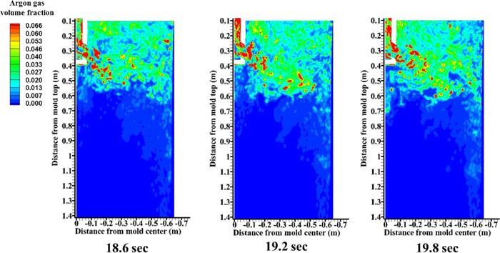
Time-averaged and instantaneous contour plots of velocity magnitude at the center plane between IR and OR in the mold are shown in Fig. 12. A classic double roll pattern is observed in the 4.8 sec time average. Two instantaneous snapshots separated by 1.2 sec show up-and-down wobbling of jet flow in the mold, which induces different impinging points of the jet onto the NF. This causes fluctuating strengths of the flow up the NF, and corresponding fluctuations of the surface flow with time. Jet wobbling also induces corresponding variations in the argon gas distribution, as shown in Fig. 13. The time-averaged flow pattern near the top surface, shown in Fig. 14, matches well with the nail board measurements in Fig. 7.Transient surface flow patterns separated by 1.2 sec show strong cross flow between the IR and the OR, which agrees with the transient surface flow patterns of the nail board measurements. According to the measurements, these surface flow variations often exceed ~200% of the mean horizontal (x-velocity) component from NF to SEN.

Fig. 12.

Time-averaged and instantaneous velocity magnitude in the mold. (Online version in color.)

Fig. 13.

Instantaneous argon gas distributions in the mold. (Online version in color.)

Fig. 14.

Time-averaged and instantaneous velocity magnitude at the surface.

5.3. Transient Velocity Variation

Instantaneous velocity magnitude histories are presented at 4 locations in the nozzle and 6 locations in the mold shown in Fig. 15. As shown in Fig. 16, points P-1 and P-2 in the nozzle have high velocity but small fluctuations, compared with P-3 and P-4 near the port, which have ~30% smaller magnitude and large fluctuations (often reaching 100% of the local mean velocity). The rotating swirl flow in the well-bottom region shown in Fig. 11 causes flow instability, and high velocity fluctuations, and appears to worse with gas injection²²⁾ and is also influenced by the backflow region and the port-to-bore ratio.^44,45) In the mold region, P-5 in the jet shows much higher velocity (~130% higher) and corresponding higher fluctuations (~200% bigger) than locations at the surface or deep in the strand, which all show fluctuations (based on standard deviations relative to the mean velocity) of ~10–30%. Point P-8 (w/4 region) midway between the SEN and the NF shows the highest average velocity (~0.34 m/sec) at the surface with fluctuations of ~15%. Computational modeling under-predicts the fluctuations, compared with the measured ~50% fluctuations observed in the nail board dipping tests.

Fig. 15.

Location of points in the nozzle and mold center-middle plane. (Online version in color.)

Fig. 16.

Transient velocity magnitude histories calculated (a) in the nozzle and (b) in the mold. (Online version in color.)

A power spectrum analysis of the velocity history was performed to evaluate the strength of different frequencies in the turbulent fluctuations, as shown in Fig. 17. The power of the fluctuations is higher at P-4 in the nozzle port than at other points in the nozzle. All nozzle points show a similar profile, with power generally decreasing with increasing frequency. In the mold regions, the jet core at P-5 shows the highest power. Surface fluctuations decrease in power according to following sequence P-7, P-6, P-9, and P-8 (P-7 > P-6 > P-9 > P-8). This is significant, because point P-8 has the highest average velocity. This suggests that surface instability cannot be predicted by examining only averages of surface quantities. The strongest fluctuation powers are generally found at the lowest frequencies, which matches previous observations.³⁵⁾ Strong peaks are observed in the nozzle and mold with various frequencies between 0.1 and 10 Hz, including several characteristic frequencies of 0.5–2 Hz at the nozzle port and jet core, due to the interaction between the strong recirculation in the nozzle bottom and the natural turbulence. These frequency ranges correspond to the time intervals of periodic momentum fluctuations in the mold (0.1 to 10 sec) and in the nozzle (0.5 to 2 sec). Recall that these frequencies are caused by transients predicted over only ~10 sec in each symmetric half of the mold. Further consideration of longer time intervals and side-to-side variations would likely induce a wider frequency range of power at the mold surface.

Fig. 17.

Power spectra calculated (a) in the nozzle and (b) in the mold. (Online version in color.)

5.4. Model Validation

The transient model of molten steel and argon gas using the coupled LES and Lagrangian DPM model was validated by comparing the predicted surface level and the surface velocity magnitude with the measurements from the nail board dipping tests. The predicted surface level profile h_steel is calculated from the surface pressure P_i , the average pressure P_Avg at the surface, and gravity acceleration g as follows⁴⁶⁾   

$${\mathrm{h}}_{\text{steel}}=\frac{{\mathrm{P}}_{\mathrm{i}}-{\mathrm{P}}_{\mathrm{A}\mathrm{v}\mathrm{g}}}{\rho \mathrm{g}}$$(23)

In this equation, slag density is not included because the slag layer experiences lifting while maintaining relatively constant thickness, rather than displacement, as observed in the measured slag motion in Figs. 4 and 5. Details of this slag layer motion behavior will be discussed further in Part II.

As shown in Fig. 18(a), the predicted surface level profiles show remarkable agreement with the measured ones. The level near the narrow face and SEN are 6–8 mm higher than the minimum level found midway in between. Both also have large variations which show evidence of transient sloshing behavior. The measured variations increase towards the SEN and the NF and are much larger than the predictions. This is likely because the measurements cover 9 minutes but the predictions only cover 3 sec. During 3 sec, the LES model can capture only the high frequency and low amplitude components of the surface fluctuations. The low frequency and high amplitude wave motion observed in the measurements would require much longer modeling time. The measured sloshing frequency is far longer than 3 sec, so cannot be captured.

Fig. 18.

Comparison of (a) surface level and (b) surface velocity between the computational modeling and the measurement. (Online version in color.)

Surface velocity predicted by the LES model is compared with the measurements in Fig. 18(b) and shows a reasonable match. The predictions are somewhat higher than the measurements, but fall within the range of the measurements. Again, it is likely that longer simulation time would produce an even better match for the velocity fluctuations. The surface velocity profile increases from less than 0.1 m/s near the SEN and NF to a maximum of over 0.3 m/sec midway between. This maximum is within the optimal range of 0.2–0.5 m/sec suggested by Kubota et al.⁴⁷⁾ to avoid defects. Of greater concern is the variability and potential sloshing, which is investigated further in Part II.

6. Conclusions

The transient fluid flow of molten steel and argon gas during steady continuous casting was investigated by employing the nail board dipping test and the LES coupled with the Lagrangian DPM.

• A series of nail board dipping tests captures level and velocity variations at the surface during nominally steady-state casting.

• The surface level profile of the molten steel shows time-variations induced by sloshing with high level fluctuations (up to ~8mm) near the SEN. In the quarter point region, located midway between the SEN and the NF, surface level is the lowest with the highest stability.

• The surface level of the liquid mold flux varies according to the lifting force produced by the molten steel motion below.

• Surface flow mostly goes towards to the SEN according to a classic double roll pattern in the mold. Transient asymmetric cross-flow between the IR and the OR mainly goes towards to the IR at the region near the OR and shows random variations (~200% of mean horizontal velocity towards the SEN) near the IR.

• The chaotic fluctuations of the surface velocity are almost 50% of the average surface velocity magnitude across the entire mold width. This finding suggests that surface velocity fluctuations are very important to understand transient surface flow phenomena resulting in defects.

• Clockwise rotating flow pattern in the nozzle well is produced by the asymmetric opening area of the middle plate of the slide-gate. When clockwise rotating flow becomes weak, small counter-clockwise rotating flow is also induced in the nozzle well.

• Up-and-down wobbling of the jet flow induces variations of velocity magnitude and direction at the surface and changes the jet flow impingement point on the NF. The jet wobbling also influences argon gas distribution with time in the mold.

• Nozzle flow shows bigger velocity fluctuation with higher power in the well and port region.

• Jet flow with high velocity fluctuations becomes slower with increasing stability after impingement on the NF, resulting in slower velocity (~60% lower) with smaller fluctuations (~70% less) at the surface.

• Strong peaks are observed at several different frequencies between 0.1 and 10 Hz (0.1 to 10 sec), including several characteristic frequencies from 0.5–2 Hz (0.5–2 sec) at the nozzle port and jet core.

• LES coupled with Lagrangian DPM shows a very good quantitative match with the average surface profile and velocities from the nail board measurements, and the trends of their fluctuations. The model under-predicts the magnitude of the measured variations of both level and velocity, likely due to the short modeling time (4.8 sec), which is insufficient to capture the important low-frequency fluctuations. Longer calculating time is needed to improve the model predictions of transient behavior.

Acknowledgements

The authors thank POSCO for their assistance in collecting plant data and financial support (Grant No. 4.0004977.01), and Mr. Yong-Jin Kim, POSCO for help with the plant measurements. Support from the National Science Foundation (Grant No. CMMI 11-30882) and the Continuous Casting Consortium, University of Illinois at Urbana-Champaign, USA is also acknowledged.

References

• 1)  World Steel in Figures 2012, World Steel Association, Brussels, Belgium, (2012).
• 2)   C.  Ojeda,  B. G.  Thomas,  J.  Barco and  J. L.  Arana: Proc. of AISTech 2007, Assoc. Iron Steel Technology, Warrendale, PA, USA, (2007), 269.
• 3)   J.  Sengupta,  C.  Ojeda and  B. G.  Thomas: Int. J. Cast Metal. Res., 22 (2009), 8.
• 4)   S-M.  Cho,  G-G.  Lee,  S-H.  Kim,  R.  Chaudhary,  O-D.  Kwon and  B.  Thomas: Proc. of TMS 2010, TMS, Warrendale, PA, USA, (2010), 71.
• 5)   S-M.  Cho,  S-H.  Kim,  R.  Chaudhary,  B. G.  Thomas,  H-J.  Shin,  W-R.  Choi and  S-K.  Kim: Iron Steel Technol., 9 (2012), 85.
• 6)   M.  Iguchi,  J.  Yoshida,  T.  Shimizu and  Y.  Mizuno: ISIJ Int., 40 (2000), 685.
• 7)   L. C.  Hibbeler,  R.  Liu and  B. G.  Thomas: Proc. of 7th ECCC, METECInSteelCon, Steel Institute VDEh, Dusseldorf, Germany, (2011).
• 8)   R.  Hagemann,  R.  Schwarze,  H. P.  Heller and  P. R.  Scheller: Metall. Mater. Trans. B, 44B (2013), 80.
• 9)   J.  Sengupta,  B. G.  Thomas,  H.  Shin,  G.  Lee and  S.  Kim: Metall. Mater. Trans. A, 37A (2006), 1597.
• 10)   H.  Shin,  S.  Kim,  B. G.  Thomas,  G.  Lee,  J.  Park and  J.  Sengupta: ISIJ Int., 46 (2006), 1635.
• 11)   N.  Bessho,  R.  Yoda and  H.  Yamasaki: Iron Steelmaker, 18 (1991), 39.
• 12)   P.  Andrzejewski,  K.-U.  Kohler and  W.  Pluschkeli: Steel Res., 3 (1992), 242.
• 13)   H.  Yu and  M.  Zhu: ISIJ Int., 48 (2008), 584.
• 14)   B. G.  Thomas,  X.  Huang and  R. C.  Sussman: Metall. Mater. Trans. B, 25B (1994), 527.
• 15)   Z.  Wang,  K.  Mukai and  D.  Izu: ISIJ Int., 39 (1999), 154.
• 16)   R.  Sanchez-Perez,  R. D.  Morales,  M.  Diaz-Cruze,  O.  Olivares-Xometl and J. P-Ramos: ISIJ Int., 43 (2003), 637.
• 17)   N.  Kubo,  T.  Ishii,  J.  Kubota and  N.  Aramaki: ISIJ Int., 42 (2002), 1251.
• 18)   V.  Singh,  S. K.  Dash,  J. S.  Sunitha,  S. K.  Ajmani and  A. K.  Das: ISIJ Int., 46 (2006), 210.
• 19)   M.  Burty,  M.  De Santis and  M.  Gesell: Rev. Metall., 99 (2002), 49.
• 20)   B. G.  Thomas and  L.  Zhang: ISIJ Int., 41 (2001), 1181.
• 21)   T.  Toh,  H.  Hasegawa and  H.  Harada: ISIJ Int., 41 (2001), 1245.
• 22)   H.  Bai and  B. G.  Thomas: Metall. Mater. Trans. B, 32B (2001), 269.
• 23)   Y.  Miki and  S.  Takeuchi: ISIJ Int., 43 (2003), 1548.
• 24)   Z.  Liu,  B.  Li,  M.  Jiang and  F.  Tsukihashi: ISIJ Int., 53 (2013), 484.
• 25)   S.  Kunstreich,  P. H.  Dauby,  S-K.  Baek and  S-M.  Lee: European Continuous Casting Conf., ATS, France, (2005), S14_12 P037.
• 26)   P. H.  Dauby: Rev. Metall., 109 (2012), 113.
• 27)   P. H.  Dauby,  W. H.  Emling and  R.  Sobolewski: Ironmaker Steelmaker, 13 (1986), 28.
• 28)   R.  McDavid: Masters Thesis, University of Illinois at Urbana-Champaign, (1994).
• 29)   R.  Liu,  J.  Sengupta,  D.  Crosbie,  S.  Chung,  M.  Trinh and  B.  Thomas: Proc. of TMS 2011, TMS, Warrendale, PA, USA, (2011).
• 30)   B.  Rietow and  B. G.  Thomas: Proc. of AISTech 2008, AIST, Warrendale, PA, USA, (2008).
• 31)   S.  Cho,  H.  Lee,  S.  Kim,  R.  Chaudhary,  B. G.  Thomas,  D.  Lee,  Y.  Kim,  W.  Choi,  S.  Kim and  H.  Kim: Proc. of TMS2011, TMS, Warrendale, PA, USA, (2011), 59.
• 32)   R.  McDavid and  B. G.  Thomas: Metall. Mater. Trans. B, 4B (1996), 672.
• 33)   W. H.  Emling,  T. A.  Waugaman,  S. L.  Feldbauer and  A. W.  Cramb: Proc. of 77th Steelmaking Conf., ISS, Warrendale, PA, USA, (1994), 371.
• 34)   H.  Bai and  B. G.  Thomas: Metall. Mater. Trans. B, 32B (2001), 253.
• 35)   R.  Chaudhary,  G-G.  Lee,  B. G.  Thomas and  S-H.  Kim: Metall. Mater. Trans. B, 39B (2008), 870.
• 36)   Q.  Yuan,  B. G.  Thomas and  S. P.  Vanka: Metall. Mater. Trans. B, 35B (2004), No. 4, 685.
• 37)   J. T.  Kuo and  G. B.  Wallis: Int. J. Multiphas. Flow, 14 (1988), 547.
• 38)   J.  Aoki,  L.  Zhang and  B. G.  Thomas: Proc. of 3rd Int. Cong. on Science & Technology of Steelmaking, AIST, Warrendale, PA, USA, (2005).
• 39)  ANSYS FLUENT 13.0-Theory Guide, ANSYS Inc., Canonsburg, PA, USA, (2010).
• 40)   H.  Bai and  B. G.  Thomas: Metall. Mater. Trans. B, 32B (2001), 1143.
• 41)   G-G.  Lee,  B. G.  Thomas and  S-H.  Kim: Met. Mater. Int., 16 (2010), 501.
• 42)   X-W.  Zhang,  X-L.  Jin,  Y.  Wang,  K.  Deng and  Z-M.  Ren: ISIJ Int., 52 (2011), 581.
• 43)   F. M.  White: Fluid Mechanics, 4th ed., Mc-Graw Hill, New York, NY, (1999).
• 44)   T.  Honeyands,  J.  Lucas,  J.  Chambers and  J.  Herberston: 75th Steelmaking Conf., ISS, Warrendale, PA, USA, (1992), 451.
• 45)   F. M.  Najjar,  B. G.  Thomas and  D. E.  Hershey: Metall. Mater. Trans. B, 26B (1995), 749.
• 46)   G. A.  Panaras,  A.  Theodorakakos and  G.  Bergeles: Metall. Mater. Trans. B, 29B (1998), 1117.
• 47)   J.  Kubota,  K.  Okimoto,  A.  Shirayama and  H.  Murakami: Mold Operation for Quality and Productivity, ed. by A.W. Cramb and E. Szekeres, ISS, Warrendale, PA, (1991).