Modelling the Evolution of Multiple Hardening Mechanisms during Tempering of Fe–C–Mn–Ti Martensite

Abstract

We model the hardness evolution of martensite during tempering as a linear addition of multiple hardening mechanisms that is combined with a microstructural Kampmann-Wagner-Numerical (KWN) model to simulate the nucleation and growth of TiC-precipitates during tempering. The combined model is fitted to the measured hardness evolution during tempering at 300°C and 550°C of martensitic steels with and without the addition of titanium. The model predicts TiC-precipitate sizes in agreement with experimental observations and generates fitting parameters in good agreement with literature. The microstructural components that give the highest contribution to the overall hardness are Fe₃C precipitates (88 HV) and dislocations (54 HV). Both Fe₃C- and dislocation-strengthening decreases rapidly during the initial stage and stabilise after 10 minutes of tempering. The model shows that the decrease in dislocation density due to recovery is slowed down due to the presence of TiC-precipitates. Titanium atoms in solid solution give a stable hardness contribution (25 HV) throughout the tempering process. TiC-precipitate strengthening generates a minor contribution (3.5 HV). The model shows that less than 1% of the equilibrium volume fraction of TiC-precipitates forms during isothermal tempering at 550°C due to the large misfit strain (1.34 GJ/m³) and a limited density of potential nucleation sites in the martensite. The model shows that the hardness of tempered martensitic steels could potentially be increased by increasing the TiC-precipitate density by reducing the misfit strain.

1. Introduction

Tempered martensitic steel is the most commonly used material for high-strength fasteners in mass-produced car engines today.¹⁾ These steels fulfil the typical requirements for the service conditions of fasteners used in current passenger cars: ultimate tensile strengths up to 1200 MPa and a recommended service temperature of max 300°C. However, the ongoing trend of engine down-sizing in order to reduce weight and CO₂-emmissions results in higher mechanical and thermal loading of the engines. Stronger and yet tough steels are now required for engine fasteners. An important boundary condition for fastener steels is a low concentration of alloying elements that are abundantly available in order to assure cost efficiency and suitability of the steel for cold forging.

The strength of martensite originates from multiple strengthening mechanisms: 1) elements in solid solution, 2) grain boundaries, 3) dislocations, and 4) precipitates.²⁾ The strength of martensite is therefore a complicated function of the martensite microstructure as this evolves during tempering of the martensite. The microstructure of martensite consists of the parent austenite grain structure which is sub-divided into packets. Each packet is divided into blocks and each block consists of parallel laths which are divided by walls of dislocations (lath boundaries).³⁾ Moreover, the microstructure of martensite consists of free dislocations, carbides, carbon atoms and other alloy atoms in solution. The carbon atoms are present in solid solution, as atoms segregated into lattice defects such as dislocations and/or as part of the different carbides. Substitutional alloying elements such as Ti are present in solid solution or in carbides.

The traditional fastener steels with strength levels up to 1200 MPa, such as 33B2 and 34Cr4, are essentially based on the first three strengthening mechanisms mentioned above. New steels for stronger fasteners have now been developed with additional strengthening from precipitates according to similar principles as used in HSLA steels.⁴⁾ Precipitates of V- and Ti-carbides are used to increase the strength to levels higher than 1200 MPa.⁵⁾ The tempering temperature which is required for the nucleation and growth of secondary V or Ti-containing precipitates is above 500°C, which fits with the requirements of the fastener standard ISO 898-1¹⁾ and the low alloy additions enable the steel to be suitable for cold forming. More importantly, TiC-precipitates have the potential to act as hydrogen traps and improve the resistance to hydrogen-induced damage⁶⁾ during processing and service of the fastener. In addition to enhancing strength, thermally stable precipitates are also known to improve the temperature resistance of steels, by acting as pinning points for movement of dislocations.⁷⁾ The high thermal stability of TiC precipitates⁸⁾ therefore makes medium-carbon steel with a small addition of Ti an interesting candidate for high-strength engine fasteners intended for service temperatures which exceed the current limit of 300°C. The mechanical properties of such fasteners will be directly related to the martensite microstructure with precipitates. Fundamental understanding of the evolution of the microstructure and the resulting hardness during tempering of martensite with small additions of Ti is required to optimise the heat treatment process and the mechanical properties of the fastener.

The aim of this study is to model the evolution of the multiple hardening mechanisms during tempering of Fe–C–Mn–Ti martensite. We simulate the hardness evolution of martensite via linear addition of the hardening mechanisms. This hardness model is combined with a microstructural multi-component and multi-phase Kampmann-Wagner-Numerical (KWN) model as developed by Den Ouden et al.,⁹⁾ for the simulation of TiC-precipitate nucleation and growth during tempering. The KWN-model takes into account the distribution of carbon atoms between phase fractions of TiC- and Fe₃C-precipitates. Moreover, the model simulates the evolution of recovery in order to estimate the effective diffusivity of Ti-atoms and in order to estimate the number of available nucleation sites for TiC-precipitates. The combined models are fitted to the experimental work of Ohlund et al. presented in Ref.¹⁰⁾.

2. Modelling the Evolution of Multiple Hardness Components during Tempering

We assume that the separate hardening mechanisms of grain size (gb), solid solution (ss), precipitates (P) and dislocations (d) can be added linearly, in agreement with:²⁾   

$${\sigma }_{tot}=\mathrm{\Delta }{\sigma }_{gb}+\mathrm{\Delta }{\sigma }_{ss}+ \mathrm{\Delta }{\sigma }_P+\mathrm{\Delta }{\sigma }_d.$$(1)

The increase of strength due to grain size is simulated by the Hall-Petch relationship is:¹¹⁾   

$$\mathrm{\Delta }{\sigma }_{gb}={\sigma }_l+k_{gb}{D}^{-1/2},$$(2)

where σ_l is the lattice friction, k_gb the Hall-Petch factor and D the average diameter of the martensite grains. D is a function of time if grain coarsening takes place.

The effective grain size of martensite is reported to be the block size.¹²⁾ A Hall-Petch term has also been suggested for the lath sub-structure within the block, but we choose to include this effect in the term for dislocation density contribution,¹³⁾ because a lath boundary can be described as a stack of dislocations.

The increase in yield strength due to elements in solid solution, i.e. C, Ti and Mn, is simulated by the general form:¹⁴⁾   

$$\mathrm{\Delta }{\sigma }_{ss,i}=K_i{c}_i^{n_i},$$(3)

where K_i is a constant for alloy element i, c_i is the concentration of element i in weight percentages and n_i is a constant that can vary from 0.5 to 2 depending on the alloying element.¹⁴⁾ The concentrations of C, Ti and Mn in the matrix are functions of time, due to redistribution into TiC and/or Fe₃C.

We set n_Mn = 1 in agreement with¹³⁾ and we assume that n_Ti = 1 due to that both Mn and Ti are substitutional atoms.

We do not include the effect of carbon atoms in solid solution in Eq. (3). Literature reports that that the well-known square root effect of carbon concentration on martensite yield strength is associated with the dislocation density of the martensite, rather than the solid solution effect of carbon atoms.^13,15) An increased carbon content of the steel generates a linear increase of the dislocation density of the quenched martensite. Carbon atoms diffuse to the Cottrell atmospheres of dislocation during quenching of the martensite and thereby maintain a higher dislocation density of the martensite, as recovery is hindered via pinning of dislocations by segregated carbon atoms. The dislocation density of martensite also generates a square root contribution to the martensite yield strength (see Eq. (5)) and the effect of increased carbon concentration on martensite therefore follows the well-established square-root dependency.

The increase in strength due to precipitates is calculated according to the Orowan-Ashby equation:¹⁶⁾   

$$\mathrm{\Delta }{\sigma }_{P,j}=\left(\frac{0.538Gb{f}_j^{1/2}}{2r_j}\right)\cdot \text{ln}\left(\frac{r_j}{b}\right),$$(4)

where G is the shear modulus of the matrix (calculated to be 80.4 GPa by a linear interpolation between the systems of Fe and Fe-1C at as concentration of 0.4 wt.%C,¹⁷⁾ b is the length of the Burgers vector (0.248 nm),¹⁸⁾ f_j is the volume fraction of precipitate phase j and r_j is the average precipitate radius of phase j (TiC and Fe₃C). f_j and r_j are functions of time due to the nucleation and growth of Fe₃C- and TiC-precipitates.

The increase in yield strength by dislocations is calculated according to¹⁹⁾   

$$\mathrm{\Delta }{\sigma }_d=M\alpha Gb{\rho }^{1/2},$$(5)

where M = 2.733 (the Taylor factor)²⁰⁾ and α (an empirical parameter) are constants. The dislocation density, ρ, is a function of time due to recovery. Recovery is in turn affected by the number of precipitates present in the material, as precipitates pin dislocations. The effect of precipitates on the recovery kinetics can be described according to¹⁹⁾ by   

$$\begin{array}{l}\frac{d\left(\mathrm{\Delta }{\sigma }_d\right)}{dt}=\left[-\frac{64{\left(\mathrm{\Delta }{\sigma }_{\rho }\right)}^2{\nu }_d}{9M^3{\alpha }^{2}E}\text{exp}\left(-\frac{U_a}{k_{B}T}\right)\text{sinh}\left(\frac{\mathrm{\Delta }{\sigma }_{\rho }{V}_a}{k_{B}T}\right)\right]\\ \left(1-\frac{N\left(t\right)}{N_c\left(t\right)}\right)\mathrm{\hspace{0.17em} }\mathrm{f}\mathrm{o}\mathrm{r}\mathrm{N}<{\mathrm{N}}_{\mathrm{c}}\mathrm{\hspace{0.17em} }\mathrm{a}\mathrm{n}\mathrm{d}\mathrm{\hspace{0.17em} }\frac{d\left(\mathrm{\Delta }{\sigma }_d\right)}{dt}=0\mathrm{\hspace{0.17em} }\mathrm{f}\mathrm{o}\mathrm{r}\mathrm{N}\ge {\mathrm{N}}_{\mathrm{c}},\end{array}$$(6)

where v_d and E are the Debye frequency and Youngs modulus respectively and α has the same meaning as in Eq. (5). U_a and V_a are the activation energy and activation volume for recovery respectively, N(t) is the number of TiC precipitates, and N_c(t) is the total number of dislocation nodes. We use the same approximation as¹⁹⁾ for the number of dislocation nodes: 0.5ρ(t)^1.5. Similar to,¹⁹⁾ we also approximate v_d and U_a using the self-diffusivity of iron in martensite²¹⁾ and the lattice parameter of martensite.²²⁾

V_a is assumed to be temperature independent. The parameters α and V_a are assumed unknown and will be fitted to the experimental data.

We use Eq. (6) to model the evolution of Δσ_d as a function of time, and we thereafter calculate ρ(t) via Eq. (5). We assume that microstructure in the as-quenched state corresponds to 0% recovery and the dislocation density ρ_AsQ in the as-quenched state is 14.2 × 10¹⁴ m^–2, as found in the literature.²³⁾

The total yield strength of each strengthening mechanism can thereafter be converted to hardness according to:²⁴⁾   

$$HV={\sigma }_{tot}/3.$$(7)

The unknown parameters in the hardness model are σ₀, K_Mn, K_Ti, α and V_a. The values for $f_{F{e}_{3}C}$ and $r_{F{e}_{3}C}$ are obtained from the experimental measurements presented in later sections. The values for f_TiC and r_TiC are obtained from simulations with the multicomponent KWN model which is discussed in the next section. The concentrations of C, Ti and Mn in solid solution can be obtained from the measured and simulated data.

3. Modelling the Nucleation and Growth of TiC-precipitates during Tempering

Literature reports that TiC precipitates in steel nucleate near dislocations²⁵⁾ and that the nucleation rate of TiC is high, followed by slower growth and coarsening.²⁶⁾ Studies have furthermore shown that both TiC nucleation and growth is enhanced by the presence of dislocations.¹⁰⁾ Literature furthermore reports that the presence of TiC precipitates in martensite affects the evolution of the dislocation density in steel during the heat treatment.^10,18) The modelling of TiC nucleation and growth in martensite must therefore be linked to dislocation density and recovery in martensite during tempering.

3.1. Nucleation of TiC

We assume that the nucleation barrier for TiC nucleation in martensite is lowered via interactions between the strain field surrounding the dislocation and the nuclei, without annihilation of the dislocation core, in agreement with.^27,28) We furthermore assume that at the moment of nucleation the TiC precipitates are coherent with the matrix in three dimensions, which implies a cubic nucleus shape.

The classical nucleation theory describes the change in Gibbs free energy associated with a nucleation event of one such cubic nucleus as:   

$$\Delta G=l^3\left(\Delta g_v+\Delta g_s\right)+6l^2{\gamma }_{eff},$$(8)

where l is the length of the sides of the cubic nuclei, Δg_v is the chemical free energy change due to the formation of the precipitate phase (also called the driving force for nucleation) which has a negative sign in case of an oversaturated matrix, Δg_s is the misfit strain energy due to the formation of the precipitate in the host lattice and γ_eff is the effective interface energy of a precipitate which interacts with a nearby dislocation strain field. The effective surface energy is calculated according to:²⁹⁾   

$${\gamma }_{eff}=\gamma -\sqrt[3]{\frac{\pi }{6}}\frac{Gb\left(1+\nu \right)}{3\pi \left(1-\nu \right)}{e}^T,$$(9)

where γ is the interface energy between TiC and ferrite (0.339 Jm^–2),³⁰⁾ G is the shear modulus of the matrix, b the Burgers vector of the dislocation, v the Poisson’s ratio of the matrix (calculated to be 0.286 by same approach as for the value of G)¹⁷⁾ and e^T is the relative lattice misfit (6% according to).³⁰⁾

The driving force for TiC-nucleation, Δg_v, is calculated by assuming a dilute solution approximation according to:⁹⁾   

$$\Delta g_v=-\frac{RT}{V_{TiC}^{mole}}{\sum }_i{x}_{TiC, i}\text{ln}\left(\frac{x_{m,i}}{x_{m,i}^{TiC/m}}\right),$$(10)

where $V_{TiC}^{mole}$ is the molar volume of TiC, x_TiC,i is the mole fraction of element i in the TiC precipitate, x_m,i the mole fraction of element i in the matrix, $x_{m,i}^{TiC/m}$ the equilibrium mole fraction of element i in the matrix at the TiC/Matrix interface and R is the gas constant.

The smallest possible nucleus of TiC is assumed to consist of one unit cell of TiC. This correspond to 14 titanium atoms, when all titanium atoms on the surface are counted as whole atoms. The length of the cube-shaped nucleus is therefore:   

$$l_{min}\ge \sqrt[3]{3.5}{a}_{TiC},$$(11)

where a_TiC = 4.33ų¹⁾ is the lattice parameter of TiC

The critical nucleus size l* is thereafter expressed by differentiation of Eq. (8) with respect to l, equating to zero and solving for l:   

$$l*=\frac{-4{\gamma }_{eff}}{\mathrm{\Delta }{g}_v+\mathrm{\Delta }{g}_s}.$$(12)

The time dependent nucleation rate of TiC precipitates, I_TiC, is expressed as:³²⁾   

$$I_{TiC}=N_{v,TiC}Z\beta *\text{exp}\left[-\frac{\mathrm{\Delta }{G}_{TiC}^{*}}{k_{B}T}\right]\text{exp}\left[-\frac{{\tau }_p}{t}\right],$$(13)

where k_B is the Boltzmann constant, T is temperature, N_v,TiC is the number density of potential nuclei sites for TiC, Z is the Zeldovich factor, β* is the frequency of atomic attachment to the growing precipitate and τ_p is the incubation time.

The number density of possible nucleation sites is as assumed to be all substitutional atomic sites within the capture radius of the dislocation:   

$$N_{v, TiC}=\pi r_c^2\rho \left(t\right)N_{v,0}.$$(14)

We use the same ρ(t) as modelled according to Eqs. (5), (6). N_v,0 is the number density of substitutional atomic sites and r_c is the capture radius of each dislocation. The capture radius of the dislocations is calculated according to:³³⁾   

$$r_c=e^{0.577}\frac{A}{4kT}\mathrm{\hspace{0.17em} }\mathrm{\hspace{0.17em} }with\mathrm{\hspace{0.17em} }\mathrm{\hspace{0.17em} }A=\frac{\mu b}{3\pi }\frac{\left(1+\upsilon \right)}{\left(1-\upsilon \right)}\mathrm{\Delta }𝕍,$$(15)

where Δ $𝕍$ is the volume difference between matrix and solute atoms.³³⁾ We calculate the volume difference between matrix and solute atoms by comparing the volume of one single Fe atom in a BCC unit cell of iron with the volume of one single Ti atom in a BCC unit cell of Ti using the lattice parameters as reported by.³⁴⁾ The capture radius as calculated from Eq. (15) is 8.7 Å at 550°C.

The Zeldovich factor is described according to:⁹⁾   

$$Z=\frac{\sqrt{2}}{\sqrt{3}}\frac{V_{TiC}^{atom}\sqrt{{\gamma }_{eff}}}{\sqrt{k_{B}T}}{\left(\frac{1}{l*}\right)}^2,$$(16)

where $V_{TiC}^{atom}$ is the atomic volume of TiC. The frequency of atomic attachment to the growing sub-critical nucleus is expressed as⁹⁾   

$$\beta *=\frac{6{\left(l*\right)}^2}{a_{TiC}^2}{\lambda }_{TiC}^m,$$(17)

where ${\lambda }_{TiC}^m$ is the effective attachment frequency of a TiC molecule, modelled as in.⁹⁾ The incubation time τ_p is given by   

$${\tau }_p=\frac{1}{2Z^2\beta *}.$$(18)

3.2. Growth of TiC

The shape of the critical nucleus is converted from a cubical to a spherical nucleus, while keeping the precipitate volume and the total Gibbs free energy constant. This leads to a critical nucleus radius r* and an effective spherical interface energy γ_r with equations:   

$$r*=\sqrt[3]{\frac{3}{4\pi }}l*\mathrm{\hspace{0.17em} }\mathrm{\hspace{0.17em} }\mathrm{a}\mathrm{n}\mathrm{d}\mathrm{\hspace{0.17em} }\mathrm{\hspace{0.17em} }{\gamma }_r=\sqrt[3]{\raisebox{1ex}{$6$}\!\left/ \!\raisebox{-1ex}{$\pi $}\right.}{\gamma }_{eff}.$$(19)

The growth of all precipitates is thereafter modelled using a Zener approach for spherical precipitates, where the growth rate, υ_TiC, of each precipitate with radius r is expressed as:³⁵⁾   

$${\upsilon }_{TiC}=\frac{D_i}{r}\frac{c_{m,i}-c_{m,i}^{TiC/m,r}}{c_{TiC,i}-c_{m,i}^{TiC/m,r}},$$(20)

where D_i is the effective diffusivity if element i in martensite, c_m,i is the concentration of element i in the matrix, c_TiC,i is the concentration of element i in the precipitate and $c_{m,i}^{TiC/m,r}$ is the concentration of element i in the matrix at the precipitate/matrix interface. All concentrations are in the units moles per m³. The above equation must be true for each of the elements C, Ti and Mn, which leads to three equations with the four unknowns υ_TiC, $c_{m,C}^{TiC/m,r}$ , $c_{m,Ti}^{TiC/m,r}$ and $c_{m,Mn}^{TiC/m,r}$ . The concentrations for iron are obtained by a mole balance.

The fourth equation needed to solve for the four unknowns is given by an adjusted form of the Gibbs-Thomson effect, which includes the effects of misfit strain energy:   

$${\sum }_{i\in \left\{Fe,C,Ti,Mn\right\}}{x}_{TiC,i}\text{ln}\left(\frac{x_{m,i}^{TiC/m,r}}{x_{m,i}^{TiC/m,\infty }}\right)=\frac{V_{TiC}^{atom}{\gamma }_r}{k_{B}T}\frac{2}{r}+\frac{V_{TiC}^{atom}}{k_{B}T}\mathrm{\Delta }{g}_s.$$(21)

This equation can be derived similar to the procedure given in.³⁶⁾ We adjust the Gibbs-Thomson effect to account for the misfit strain energy to obtain consistency between the nucleation part of the model and the growth part of the model: if the Gibbs-Thomson effect is not adjusted for the effect of the misfit strain energy, a precipitate with zero growth rate, i.e. v_TiC = 0, will have a radius unequal to r*, which is physically incorrect.

Earlier studies have shown that the high dislocation density of martensite increases the diffusion rate in martensite.¹⁰⁾ The effective diffusivities of C, Ti and Mn in martensite, 〈D_C〉, 〈D_Ti〉, 〈D_Mn〉, are therefore taken as a balance between the lattice diffusivities, $D_L^{C/M}$ , $D_L^{Ti/M}$ , $D_L^{Mn/M}$ , and the pipe diffusivities, $D_p^{C/M}$ , $D_p^{Ti/M}$ , $D_p^{Mn/M}$ , on the format given by³⁷⁾ where we remove the cross section area for pipe diffusivity from the area of lattice diffusivity:   

$$⟨D_e⟩=\left(1-g\left(t\right)\right)D_L^{e/M}+g\left(t\right)D_p^{e/M}\mathrm{\hspace{0.17em} }\mathrm{\hspace{0.17em} }\mathrm{f}\mathrm{o}\mathrm{r}\mathrm{\hspace{0.17em} }\mathrm{\hspace{0.17em} }e=C,Ti,Mn.$$(22)

Here g(t) is the cross sectional area of dislocation pipe per unit area of matrix.

The pipe diffusivities for Ti and Mn are unknown, but under the assumption that the presence of a dislocation lowers the energy barrier for diffusion, it is reasonable to assume that the ratio between the bulk diffusivities and the pipe diffusivities of the elements C, Ti and Mn is equal to the ratio between the bulk diffusivity and pipe diffusivity of Fe:   

$$\frac{D_p^{e/M}}{D_L^{e/M}}= \frac{D_p^{Fe/M}}{D_L^{Fe/M}}\mathrm{\hspace{0.17em} }\mathrm{\hspace{0.17em} }\mathrm{f}\mathrm{o}\mathrm{r}\mathrm{\hspace{0.17em} }\mathrm{\hspace{0.17em} }e=C,Ti,M,$$(23)

where the ratio $\frac{D_p^{Fe/M}}{D_L^{Fe/M}}$ is found in.²¹⁾ The effective pipe radius of a dislocation is set equal to the Burgers vector, b, and the cross sectional area of dislocation per unit area of matrix is expressed as:   

$$g\left(t\right)=\rho \left(t\right)\pi b^2.$$(24)

The number balance of precipitates in the model is described according to⁹⁾   

$$\frac{\partial \varphi }{\partial t}=-\frac{\partial \left[v_{TiC}\varphi \right]}{\partial r}+\delta \left(r-r_{k_{B}T}^{*}\right)I_{TiC},$$(25)

in which ϕ ≡ ϕ(r,t) in m^–4 is the number density distribution of precipitates of radius r at time t and v_TiC in ms^–1 represents the growth rate of precipitates of radius r at time t. The radius $r_{k_{B}T}^{*}$ is the radius for which the energy of nucleation is k_BT less than the energy for r* ( $r_{k_{B}T}^{*}$ > r*).

The key features of the model for TiC precipitation⁹⁾ are the inclusion of multi-component and multi-phase effects within the model. In⁹⁾ it has been shown that the model is capable of dealing with the multiple secondary phases which compete for the same solid solution elements.

We choose a different numerical method than that from.⁹⁾ We use a combination of Strang splitting, first-order upwinding,³⁸⁾ Implicit and Explicit Euler time-integration and adaptive mesh techniques. The initial mesh contains 500 bins on a logarithmic scale, similar to.⁹⁾ The simulation is following the same temperature profile as applied directly after quenching during the experiments of Ohlund et al.¹⁰⁾

4. Experimental

We have published the experimental methods and results elsewhere before.¹⁰⁾ The experimental results are now being used as input parameters and validation for the proposed model. Two high-purity Fe–C–Mn steels are investigated: one without Ti and one with the addition of 0.042 wt.% Ti. The compositions of the steels are given in Table 1. The Ti-free steel is austenitised at 940°C for 40 minutes and the Ti-containing steel is homogenised and austenitised at 1350°C for 30 minutes. The austenisation temperature of 1350°C is chosen to assure that all Ti atoms are in solid solution. The different austenisation times are chosen to obtain similar austenite grain sizes. Both steels are quenched to room temperature from their respective austenisation temperature, using He-gas followed by tempering treatments performed at 300°C and 550°C for 5, 10, 30 and 60 minutes. The heating time up to the full tempering temperature is 138 seconds. The tempering temperature of 300°C is chosen to assure that all Ti atoms remain in solid solution, as nucleation of TiC does not take place during tempering at 300°C.⁶⁾ The tempering level of 550°C is chosen to assure that TiC nucleation and growth takes place during tempering, as literature report that TiC nucleation take place when tempering temperatures are in the range of 550°C.⁶⁾

Table 1. Chemical composition of the examined steels (wt%).

Steel	C	Mn	Si	P	S	Al	Ti	Cu	Cr	O	V
Ti-free	0,39	0,8700	0,0035	0,0010	0,0007	0,0050	–	0,0012	0,0018	0,0080	0,0023
Ti-containing	0,39	0,8700	0,0040	0,0011	0,0007	0,0047	0,0420	0,0012	0,0022	0,0046	0,0022

Micro-Vickers hardness (HV0.5) is used to study the evolution of macroscopic hardness. Scanning electron microscopy (SEM, JEOL JSM-6500F with field emission gun) is used to study the evolution of Fe₃C-particle size and volume fraction. Electron back-scatter diffraction (EBSD with a Nordlys detector) is used to study the coarsening of martensite blocks and to estimate the evolution of recovery in the martensite. We estimate the evolution of recovery from the crystallographic indexing results. Block boundaries, high surface roughness, high elastic strain and high strain levels due to e.g. dislocations reduces the band contrast of the Kikuchi patterns of the EBSD signal. If the degradation is high enough, the measurement point cannot be indexed. As no block coarsening takes place during annealing and the surface roughness and elastic strain is comparable for all specimens, we consider the improvement of the band contrast during annealing to be a result of recovery. However, since only regions close to block boundaries contain dislocation densities which are high enough to prevent indexing in the as quenched state, the results are only representative for regions adjacent to block boundaries. The indexing results for the as-quenched specimen is considered to be representative for martensite with no recovery and the indexing results for the specimens tempered for 60 minutes is considered to be representative for the fully recovered state. The dislocation density in the as quenched state is set to the value measured by Morito et al.²³⁾ and the dislocation density in the fully recovered state after annealing is given by Takebayashi et al.³⁹⁾ The indexing result is thereafter used to estimate the recovery evolution and the dislocation density during annealing.

Atom probe tomography (APT, Imago LEAP 3000X HR with laser pulsing) is used to measure the concentration of carbon and titanium atoms in solid solution and the TiC-precipitates in the Ti-containing martensite after 60 minutes of tempering at 550°C.

5. Model Fitting

5.1. Input Parameters

The EBSD measurements in Ref.¹⁰⁾ show that no grain coarsening takes place during tempering. Therefore, we take Δσ_gb in Eq. (2) as a constant.

The measured volume fraction of Fe₃C-particles as a function of annealing time and temperature is used as an input to the model. The SEM-measurements in Ref.¹⁰⁾ are used to determine the Fe₃C-particle width, w, and length, l, which are used to calculate the volume fraction of Fe₃C precipitates. We calculate the volume of each Fe₃C-particle that is measured within a square area of SEM images using   

$$V=4\pi {\left(\frac{w}{2}\right)}^2\left(\frac{l}{2}\right).$$(26)

The total volume of all particles is summarized within each sample. The volume fraction of Fe₃C-precipitates as a function of annealing time and temperature is determined, assuming a cubic measurement volume. We observe that the equilibrium volume fraction of Fe₃C-precipitates is 0.087 for the Ti-containing steel after 60 minutes of isothermal tempering at 550°C. However, ThermoCalc simulations (TCFE6) for the Ti-containing steel show that the equilibrium volume fraction of Fe₃C is equal to 0.058 at 550°C. The higher volume fraction we measure from SEM can be due to a slight overestimation of particle dimensions from SEM pictures and due to the assumption of oval particle shape (Eq. (26)). We now use the APT measurements to estimate the volume fraction of Fe₃C in the Ti-containing steel after 60 minutes of tempering at 550°C. The APT measurement show that the concentration of carbon atoms in solid solution is 35·10^–3 at% C. This is higher than the simulated equilibrium concentration of C atoms in solid solution in ferrite at 550°C (1.8·10^–3 at% according to ThermoCalc). From the APT results we can also estimate the fraction of carbon atoms that is used for the formation of TiC-precipitates. We assume that carbon is distributed between TiC, Fe₃C and C in solid solution and derive that the volume fraction of Fe₃C is 0.057 (98% of the equilibrium volume fraction) after 60 minutes of isothermal tempering at 550°C.

We therefore create a scale factor from the relationship we find between the SEM and APT volume fractions for the Ti-containing steel after 60 minutes of tempering at 550°C. The volume fraction of Fe₃C, as determined by SEM, is thereafter scaled for each examined specimen.

The effective radius of the Fe₃C-particles is also used as an input parameter to the model. The effective radius of the Fe₃C-particles in each specimen is calculated from the scaled SEM volume fraction of Fe₃C by assuming spherical particles.

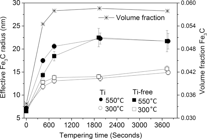
Figure 1 shows the effective Fe₃C radius and volume fraction of Fe₃C, as a function of tempering time, that are used as input parameters in the model. The four curves for volume fraction of Fe₃C are overlapping, and we therefore show only the Ti-containing steel at 550°C. Both the effective precipitate size and the volume fraction of Fe₃C grow rapidly during the first 5 minutes of isothermal tempering. After 5 minutes of isothermal tempering the growth continues at a lower rate, and after 10 minutes the values stabilises. We note that the spread in cementite particle size increases with tempering time, during tempering at 550°C, which is reflected by the increase in the size of error bar for the average cementite particle size.

Fig. 1.

Effective Fe₃C radius [nm] of Ti-free and Ti-containing martensite during annealing at 300 and 550°C and the volume fraction of Fe₃C in the Ti-containing steel during annealing at 550°C, as a function of annealing time. Error bars represent 95% confidence interval.

The small carbides which are observed in the as-quenched state could correspond to ε-carbides, based on their size and that they are present directly after quenching. In the present model, all the iron-carbides are modelled as Fe₃C-particles. The volume fraction of Fe₃C is used to calculate the input parameter of carbon concentration in solid solution to the model, as only one data point for the carbon concentration in solid-solution was measured by APT (at 60 minutes of isothermal tempering at 550°C for the Ti-containing steel).

5.2. Fitting Approach

The parameters σ_gb, K_Mn, K_Ti, α and V_a of the hardness model are currently unknown. Two of these parameters, α and V_a, are also used within the KWN TiC precipitation model, together with the misfit strain energy Δg_s for the TiC precipitates. We will use the following approach to obtain estimates of these parameters:

1. σ_gb, K_Mn, K_Ti, α and V_a are fitted using least-squares techniques by minimising the residual between the simulated hardness given by Eqs. (1) and (7) of the model and the measured hardness from experiments. We simultaneously fit the model to the experimental data from the Ti containing steel at 300°C and the Ti free steel at 300°C and 550°C at 0, 5, 10, 30 and 60 minutes of tempering. The Ti-containing steel heat-treated at 550°C is excluded from the fitting of the above parameters in order to avoid the influence of TiC precipitates.

2. Δg_s is obtained by using a least-squares techniques by minimising again the residual between the predicted hardness and the measured hardness, where the values for the parameters σ_gb, K_Mn, K_Ti, α and V_a from the previous step are used within the hardness model and the TiC precipitation model. Only the data for the Ti-containing steel during tempering at 550°C after 0, 5, 10, 30 and 60 minutes is used to obtain the value of Δg_s.

6. Results and Discussion

6.1. Fitting Parameters

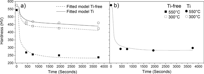
Figure 2 shows the measured hardness (symbols) and the fitted (lines) hardness as a function of annealing time of a) the Ti-free steel at 300°C and 550°C and the Ti-containing steel at 300°C and b) the Ti-containing steel at 550°C. The comparison between the experiment and the model in Fig. 2(a) is used to obtain values for the fitting parameters σ_gb, K_Mn, K_Ti, α and V_a. The comparison between the experiment and the model in Fig. 2(b) is used to fit a value for the strain energy. From Figs. 2(a) & 2(b). it can be seen that the fitted model correctly describes the evolution of the hardness during tempering. The fitted parameters σ_gb, K_Mn, K_Ti, α, V_a, and Δg_s are given in Table 2.

Fig. 2.

The measured hardness (symbols) and the fitted model (lines) of a) the Ti-free steel at 300°C and 550°C and the Ti-containing steel at 300°C as a function of annealing time and b) the Ti containing steel at 550°C. 95% confidence intervals are covered by the symbols. The error bars (representing 95% confidence intervals) are smaller than the symbols size.

Table 2. Results from least-squares fitting of Eqs. (1), (2), (3), (4), (5), (6), (7) to the measured hardness.

Parameter	Value
σgb (MPa)	340
KMn (MPa (wt%)–1)	0
KTi (MPa (wt%)–1)	1679
α	0.401
Va(m3)	16.99b3
Δgs(GJ/m3)	1.34

In the following section we compare the values of the fitted parameters to the values reported in literature. The σ_gb of our model is the combination of lattice friction and the hardness contribution of the martensite block structure (grain size hardening). The model predicts Δσ_gb = 340 MPa (113 HV). This calculated value is lower than the value of 413 MPa which is given in literature.²⁾ This difference can be due to the difference in grain size that we use and the grain size that is used in literature. The literature value of 413 MPa is based on the grain size the average lath width of 0.25 μm. This is smaller than the effective grain size (determined by the block boundaries) that we used in our model. The value that we find for α = 0.401 is in good agreement with the literature reports ranging from 0.24 to 1.^18,40) We note that the experimental work of¹⁰⁾ show that the concentration of carbon atoms in true solid solution (between laths) and the concentration of carbon atoms segregated to lath boundaries (high dislocation density) are 0.005 wt% and 0.045 wt% respectively, after 60 minutes of tempering at 550°C. This indicates that the majority of carbon atoms in the martensite have segregated to dislocations and that Eq. (5) therefore covers the major influence of carbon atoms in solid solution on the martensite strength.

The activation volume of the recovery process in martensite, V_a is compared to the literature value for the activation volume of the recovery process in BCC iron. Our model predicts a value of 17b³ or 0.26 nm³, which is in good agreement with the reported value of 0.1 to 0.6 nm³.⁴¹⁾

The fitted values of the K_Mn-parameter is zero, whereas literature reports a value of K_Mn = 35 MPa(wt%)^–1.¹³⁾

The difference between our fitted value of K_Mn = 0 and the literature value of K_Mn = 35 MPa(wt%)^–1, falls within the uncertainties of our experiments and the uncertainties of the experiments reported in literature. We estimate that Mn in solid solution contributes with maximum 10 HV to the total hardness in our system. Here we assume that the Mn-atoms do not have time to redistribute during the formation of cementite so that the overall manganese concentration in the matrix corresponds to the overall concentration of 0.87 wt% Mn in the steel. The strengthening effect of Mn in solid solution in the as-quenched martensite is therefore approx. 30 MPa (or 10 HV), in case we use the literature value for K_Mn = 35 MPa(wt%)^–1 and Eq. (3). In case the Mn-atoms would redistribute into cementite, the Mn-concentration in the matrix would be even lower and subsequently the added strength would be lower. The error in our hardness measurements is approx. ±5 HV. The steels used by¹³⁾ contain sulphur, which may form MnS precipitates. The formation of MnS can influence the hardness by precipitate strengthening and the literature value of 35 MPa(wt%)^–1 for K_Mn may therefore be biased.

There are not many reports in the literature about the strain energy if TiC-precipitates in martensite. Jang et al.³⁰⁾ have used first principles calculations to estimate a value of 4.10 kJ/mol or 1.16 GJ/m³. This value corresponds well to our fitted value of 1.34 GJ/m³ or 4.74 kJ/mol.

6.2. TiC-precipitates and Recovery

Figure 3 shows the calculated TiC precipitate size distribution together with the TiC precipitate sizes measured by Ohlund et al.¹⁰⁾ The precipitate size as measured by APT is based on the APT atom count for each precipitate¹. The KWN model predicts that 0.27% of the equilibrium volume fraction of TiC forms and that the average TiC precipitate radius is 1.38 nm after 60 minutes of isothermal tempering at 550°C. Furthermore, the model predicts that nucleation of TiC precipitates starts during the heating stage, 10 seconds before reaching the isothermal temperature of 550°C and that the peak in number density of TiC-precipitates is reached after 385 seconds of heating and tempering (after 4 minutes and 7 seconds of isothermal tempering). The predicted average radius and size distribution from the KWN model are slightly higher than the values measured by APT. However, the measured precipitates sizes fall within the nonzero part of the predicted distribution and is therefore in agreement with the model. The predicted volume fraction of formed TiC-precipitates is lower than what is measured by APT. This could be due to the small sample size inherent to APT.

Fig. 3.

The simulated TiC precipitate size distribution (line) and the experimental precipitate sizes (symbols) as measured by APT in the Ti-containing martensite after 60 minutes of tempering at 550°C.

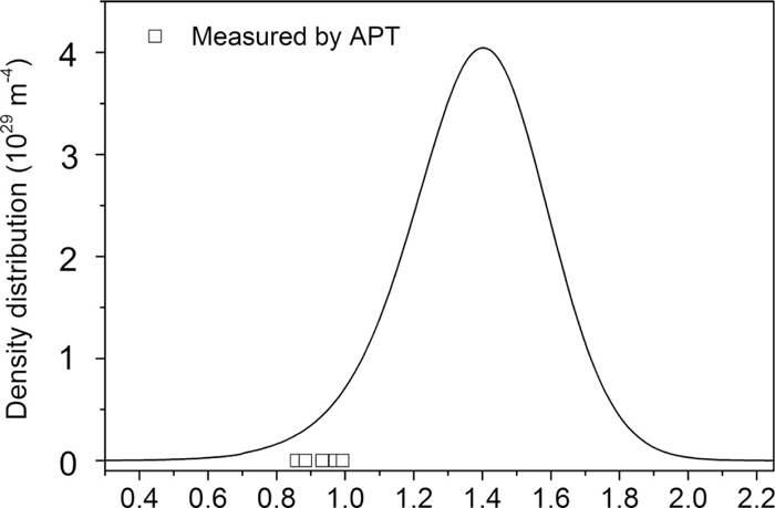
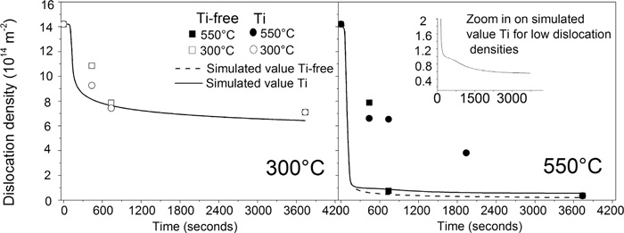
Figure 4 shows the dislocation density as a function of tempering time for Ti-free (precipitate free) and Ti-containing steel at different temperatures, as simulated via Eqs. (5), (6) and as measured by EBSD experiments.¹⁰⁾

Fig. 4.

The measured (symbols) and the simulated (lines) dislocation density in Ti-free and Ti-containing steel as a function of annealing time during annealing at 300°C and 550°C. The simulated value of Ti-containing and Ti-free steel overlap at 300°C.

We use the simulated dislocation density as input to our model. The simulation of the evolution of the dislocation density does not take into consideration the pinning of dislocations by small iron carbides and cementite particles. We observe that these type of particles are present in the steels after quenching and at all annealing times. The pinning of dislocations by iron carbides is therefore expected to be approximately constant throughout the annealing of the steels and our simulation might overestimate the amount of recovery which has occurred at times between 5 to 60 minutes of isothermal tempering.

Figure 4(a) shows the dislocation density of Ti-free and Ti-containing martensite during tempering at 300°C (where no TiC precipitates are present). We observe that the evolution of the recovery is slightly faster in the simulated values than in the experimental values and that the simulation results in a higher degree of recovery. Figure 4(b) shows the dislocation density of Ti-free and Ti-containing martensite during tempering at 550°C. We observe that the simulated and the experimental values do not correlate. The simulation of recovery in the Ti-containing steel shows faster recovery and a much higher degree of recovery than the experimental values. However, we observe a recovery delay in the simulated values, with a maximum delay effect between 200 and 550 seconds of tempering. We note that the recovery delay of the simulated dislocation density and the recovery delay observed by experiments show a similar evolution in time (see the zoomed in panel). The recovery delay of the simulations of the Ti-containing steel at 550°C results in a slightly higher dislocation density in the Ti-containing steel than in the Ti-free steel during isothermal annealing at 550°C.

The recovery delay of the simulated dislocation density is a result of the high number of TiC-precipitates which are present at that time. The KWN model predicts that the highest number of TiC precipitates, which can act as pinning points for dislocations, appears after 385 seconds of tempering. The large disagreement between simulated and experimentally estimated values at 550°C is a result of that the experimentally established recovery is representative for regions close to block boundaries. Nucleation of TiC is faster in the regions close to block boundaries, which reduces the rate of recovery in these regions.¹⁰⁾ The experimentally estimated dislocation density therefore becomes too high.

¹  We convert the atom count to a radius, assuming spherical precipitates, by the volume estimated from the lattice parameter of TiC. We add the distance of one Ti atom radius to the calculated radius as the volume estimated by the lattice parameters only measure to the centre of the outer atoms.

6.3. Evolution of Multiple Hardness Components during Tempering

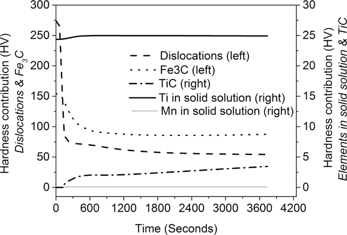
Figure 5 shows the evolution of the hardness contribution from different microstructural components of the martensite as a function of time during tempering at 550°C.

Fig. 5.

The evolution of the contribution of multiple hardness components to the overall hardness of martensite as a function of time during tempering at 550°C.

The microstructural components which give the largest direct contributions to the overall hardness of martensite during tempering are 1) Fe₃C precipitates and 2) dislocations.

The strengthening effect of Fe₃C precipitates is decreasing by 50 HV during heating to 550°C and the first 8 minutes of isothermal tempering at 550°C. This rapid decrease takes place due to the fast coarsening of Fe₃C particles during the same time period, as presented in Fig. 1. After 8 minutes of isothermal tempering the strengthening effect stabilises and our hardness model predicts that the hardness contribution of Fe₃C is approx. 88 HV, which remains stable from 8 to 60 minutes of isothermal annealing at 550°C. The high hardness contribution of Fe₃C by precipitation strengthening is supported by the literature: ε-carbides that form during low temperature annealing or during auto-tempering, have been measured to significantly increase the hardness of lath martensite.⁴²⁾ Small iron-carbides can therefore be a very effective way of increasing the strength and hardness of martensite. However, the strengthening effect of iron carbides could be sensitive to long time service at elevated temperatures due to rapid diffusion of carbon atoms, which could enable cementite coarsening via Ostwald ripening. As coarsening proceeds, the spread in particle size will increase (but the average size might remain constant). At a certain critical point, all small precipitates are consumed and the average precipitate size increases, while the number density decreases. This change in precipitate size and number of precipitates will lead to a reduction in the precipitation strengthening effect of Fe₃C. The experimental results show that the spread in cementite particle size increases with annealing time (see Fig. 1).

The strengthening effect of dislocations decreases very rapidly by approx. 200 HV during the 138 seconds of heating to the isothermal annealing temperature. This rapid decrease is a result of the rapid recovery which is shown in Fig 4(b). The strengthening effect of dislocations stabilises during tempering. Our hardness model predicts that the hardness contribution of dislocations is approximately stable at 54 HV from 10 to 60 minutes of isothermal tempering at 550°C.

The microstructural components which give minor direct contributions to the overall hardness of martensite are 1) Ti atoms in solid solution and 2) TiC, as shown in Fig. 5.

The strengthening due to Ti in solid solution increases slightly during heating up and the first minutes of isothermal tempering at 550°C and is thereafter stable. The hardness increases slightly due to a slight increase in the concentration of Ti atoms in the matrix as a result of formation of Fe₃C which redistributes a high number of Fe and C atoms from the matrix to Fe₃C. ThermoCalc simulations show that Ti does not dissolve in Fe₃C and is therefore remaining in the matrix. Our hardness model predict that the hardness contribution due to Ti in solid solution is approx. 25 HV after 60 minutes of isothermal tempering at 550°C.

The strengthening effect of TiC precipitates is zero during the majority of the heating up of the steel, and is thereafter increasing rapidly during the first 7 minutes of isothermal tempering at 550°C. After 8 minutes of isothermal tempering the hardness increases slowly. The hardness model predicts that the strengthening effect due to precipitation strengthening of TiC is approximately 3.5 HV after 60 minutes of isothermal tempering at 550°C. We note that the theoretical maximum precipitation strengthening effect of TiC is 42 HV.

The direct strengthening effect of Mn atoms in solid solution is zero during the entire process of tempering, as shown in Fig. 5.

The microstructural components which give combined contributions to the overall hardness of martensite are TiC precipitates combined with dislocations.

Our model predicts that the recovery process in the Ti containing steel is delayed during isothermal tempering at 550°C as a result of TiC precipitates which pin dislocations (see Fig. 4(b)). The resulting dislocation density of the Ti containing steel is therefore higher than the dislocation density of the Ti-free steel. This higher dislocation density contributes to a 20 HV higher hardness contribution in the Ti-containing steel after 60 minutes of isothermal tempering at 550°C, as compared to the Ti-free steel. The total strength contribution due to formation of TiC in martensite is therefore the sum of the TiC precipitation strengthening effect, and the extra dislocation strengthening effect due to less recovery. Our hardness model predicts that this combined strengthening effect is 23.5 HV after 60 minutes of isothermal tempering at 550°C.

The low strengthening effect of TiC-precipitates is a result of the low volume fraction of TiC-precipitates that is predicted by our model. We note that when the model is run for longer holding times at 550°C, there is only a slight increase in the volume fraction of formed TiC-precipitates. The resulting hardness increase is small: 5.9 HV after three hours of isothermal annealing at 550°C. An extended heat treatment time will therefore not improve the properties of the martensite by much.

The low volume fraction of TiC-precipitates is related to the large misfit strain (1.34 GJ/m³) that we find during fitting and the low density of potential nucleation sites (Eq. (14)) that we use as input parameter to the model. Both factors reduce the nucleation rate. The low density of potential nucleation sites is a result of the rapid recovery of the simulated dislocation density which is used as an input to our model, and the calculated capture radius.

We investigate the influence of a higher number of available nucleation sites by repeating the fitting of our model to the measured hardness at 550°C, using 1) a increased capture radius of 2·r_c, as calculated by Eqs. (15) and (2) a higher dislocation density of the martensite. To increase the dislocation density we use the experimental dislocation density of Fig. 4(b) as input to the model, instead of simulating the dislocation density according to Eqs. (5), (6) within the model.

We investigate the effect of lower mis-fit strain by setting a fixed value of the mis-fit strain (75% of the value predicted by our fit to the measured hardness) as input parameter to the model. We investigate the effect of a lower mis-fit strain energy combined with a higher number of available nucleation sites, by setting the mis-fit strain energy to 1.3359 GJ/m³ and using the experimental dislocation density as input parameters to the KWN model. The results from the repeated fit of our model and the accuracy of the simulated values to the measured hardness (given as the sum of squared errors) are given in Table 3, together with the values from our original fitting.

Table 3. Results from least-squares fitting of model, using modified input parameters.

Modified input parameter	fTiC	Accuracy of model	Δgs
Original model (no modification)	0.27%	793	1.3359 GJ/m3
Capture radius 2⋅rc	0.28%	788	1.3347 GJ/m3
Higher dislocation density (Experimental result)	0%	41638	2.3189 GJ/m3
Δgs = 1.0019 GJ/m3	17%	973
Higher dislocation density & Δgs = 1.3359 GJ/m3	44.9%	1.336 × 109

An increased capture radius does not generate a higher volume fraction of TiC-precipitates, but it slightly improves the accuracy of the fitting of the model. Increasing the dislocation density alone results in a considerably higher value for the misfit strain energy after fitting, which does not correspond anymore to first-principles calculations.³⁰⁾ Moreover, in this case the model predicts that no nucleation of TiC-precipitates takes place. A reduction of the misfit strain energy results in a higher volume fraction of formed TiC, and a slight reduction of the accuracy of the fit. A reduction of the mis-fit strain energy and a higher dislocation density results in a significantly increased volume fraction of TiC-precipitates and a smaller precipitate size. The latter results are more in agreement with the APT measurement. However, the model is no longer capable of fitting to the measured hardness.

7. Conclusions

We quantify the evolution of the multiple hardness contributions to the overall hardness of martensite containing TiC-precipitates during isothermal annealing. We simulate the hardness of martensite as a linear addition of multiple hardening mechanisms. This hardness model is combined with a microstructural model based on the Kampmann-Wagner-Numerical (KWN) approach for a multi-component and multi-phase system to simulate the nucleation and growth of TiC-precipitates.

The two microstructural components which contribute most to the overall hardness of the investigated Fe–C–Mn–Ti steel are Fe₃C precipitates (88 HV) and dislocations (54 HV). Both contributions decrease rapidly during initial stages of annealing and stabilise after 10 minutes of annealing. The addition of titanium to the steel gives a minor hardness contribution via Ti-atoms in solid solution and TiC precipitates. Ti atoms in solid solution give a hardness contribution which increases slightly during the first minutes of annealing and thereafter remains stable (at 25 HV). The direct contribution of TiC precipitates to the overall hardness is limited (3.5 HV). However, TiC-precipitates also contribute to the overall hardness by pinning of dislocations during the recovery that takes place during the tempering. The model predicts that only a small volume fraction of TiC-precipitates forms during isothermal annealing at 550°C due to the large misfit strain (1.34 GJ/m³) and the low density of potential nucleation sites.

Acknowledgements

The authors wish to acknowledge the financial support from Koninklijke Nedschroef Holding B.V.

Part of this research was carried out under the Project number M41.5.09341 in the framework of the Research Program of the Materials innovation institute M2i (www. m2i.nl).

References

• 1)  International Organization for Standardization: ISO898-1, Mechanical Properties of Fasteners Made of Carbon Steel and Alloy Steel-Part 1, 5th ed., ISO, Geneva, (2013).
• 2)   G.  Krauss: Mater. Sci. Eng. A, 273–275 (1999), 40.
• 3)   S.  Morito,  X.  Huang,  T.  Furuhara,  T.  Maki and  N.  Hansen: Acta Mater., 54 (2006), 5323.
• 4)   T. N.  Baker: Mater. Sci. Technol., 25 (2009), 1083.
• 5)   Y.  Namimura,  N.  Ibaraki,  W.  Urushihara and  T.  Nakayama: Wire J. Int., 36 (2003), 62.
• 6)   F. G.  Wei,  T.  Hara,  T.  Tsuchida and  K.  Tsuzaki: ISIJ Int., 43 (2003), 539.
• 7)   F.  Abe,  M.  Taneike and  K.  Sawada: Int. J. Press. Vessel. Pip., 87 (2007), 3.
• 8)   M.  Taneike,  M.  Fujitsuna and  F.  Abe: Mater. Sci. Technol., 20 (2004), 1455.
• 9)   D.  den Ouden,  L.  Zhao,  C.  Vuik,  J.  Sietsma and  F. J.  Vermolen: Comp. Mater. Sci., 79 (2013), 933.
• 10)   C. E. I. C.  Ohlund,  J.  Weidow,  M.  Thuvander and  S. E.  Offerman: ISIJ Int., 54 (2014), 2890.
• 11)   L. H.  Friedman and  D. C.  Chrzan: Phys. Rev. Lett., 81 (1998), 2715.
• 12)   T.  Ohmura,  K.  Tsuzaki and  S.  Matsuoka: Scr. Mater., 45 (2001), 889.
• 13)   L. A.  Nordstrom: Scand. J. Metall., 5 (1976), 159.
• 14)  Martensite, ed. By G. B. Olsen and W. S. Owen:  ASM  International, Materials Park, Ohio, (1992), 282.
• 15)   M.  Kehoe and  P. M.  Kelley: Scr. Metall., 4 (1970), 473.
• 16)   T.  Gladman: The Physical Metallurgy of Microalloyed Steels, The University press, London, (1997), 52.
• 17)   G. R.  Speich,  A. J.  Schwoeble and  W. C.  Leslie: Metall. Trans., 3 (1972), 2031.
• 18)   Y.  Han,  J.  Shi,  L.  Xu,  W. Q.  Cao and  H.  Dong: Mater. Sci. Eng. A, A530 (2011), 643.
• 19)   H. S.  Zurob,  C. R.  Hutchinson,  Y.  Brechet and  G.  Purdy: Acta Mater., 50 (2002), 3075.
• 20)   J. M.  Rosenberg and  H. R.  Piehler: Metall. Trans., 2 (1971), 257.
• 21)   Y.  Shima,  Y.  Ishikawa,  H.  Nitta,  Y.  Yamazaki,  K.  Mimura,  M.  Isshiki and  Y.  Iijima: Mater. Trans., 43 (2002), 173.
• 22)   L.  Cheng,  C. M.  Brakman,  B. M.  Korevaar and  E. J.  Mittemeijer: Metall. Trans. A., 19(1988), 2415.
• 23)   S.  Morito,  J.  Nishikawa and  T.  Maki: ISIJ Int., 43(2003), 1475.
• 24)   B.  Huthcinson,  J.  Hagstrom,  O.  Karlsson,  D.  Lindell,  M.  Tornberg,  F.  Lindberg and  M.  Thuvander: Acta Mater., 59 (2011), 5845.
• 25)   Z.  Wang,  X.  Mao,  Z.  Yang,  X.  Sun,  Q.  Yong,  Z.  Li and  Y.  Weng: Mater. Sci. Eng. A, A529 (2011), 459.
• 26)   M.  Sawahata,  M.  Enomoto,  K.  Okuda and  T.  Yamashita: Tetsu-to-Hagané, 94 (2008), 21.
• 27)   S. Q.  Xiao and  P.  Haasen: Scr. Metall., 23 (1989), 365.
• 28)   S. Y.  Hu and  L. Q.  Chen: Acta Mater., 49 (2001), 463.
• 29)   H. I.  Aaronsons,  M.  Enomoto and  J. K.  Lee: Mechanisms of Diffusion Phase Transformations in Metals and Alloys, CRC Press, Boca Raton, (2010), 211.
• 30)   J. H.  Jang,  C. H.  Lee,  Y. U.  Heo and  D. W.  Suh: Acta Mater., 60 (2012), 208.
• 31)   A.  Teresiak and  H.  Kubsch: NanoStruct. Mater., 6 (1995), 671.
• 32)   J. W.  Cahn: Acta Metall., 4 (1956), 449.
• 33)   Z. M.  Wang and  G. J.  Shiflet: Metall. Mater. Trans. A, 29A (1998), 2073.
• 34)   D. S.  Rickerby: Met. Sci., 16 (1982), 495.
• 35)   C.  Zener: J. Appl. Phys., 20 (1949), 950.
• 36)   M.  Perez: Scr. Mater., 52 (2005), 709.
• 37)   D. A.  Porter and  K. E.  Easterling: Phase Transformations in Metals and Alloys, Van Norstrand Reinhold, New York, (1981), 102.
• 38)   R.  LeVeque: Finite Volume Methods for Hyperbolic Problems, Camebridge Univeristy Press, New York, (2002), 378.
• 39)   S.  Takebayashi,  T.  Kunieda,  N.  Yoshinaga,  K.  Ushioda and  S.  Ogata: ISIJ Int., 50 (2010), 875.
• 40)   R.  Lagneborg and  B.  Bergman: Met. Sci., 10 (1976), 20.
• 41)   A.  Smith,  H.  Luo,  D.  Hanlon,  J.  Sietsma and  S.  Van der Zwaag: ISIJ Int., 44 (2004), 1188.
• 42)   R. N.  Caron and  G.  Krauss: Metall. Trans., 3 (1972), 2381.