2. Experimental and Regression Procedures
The chemical compositions of the studied steels are listed in Table 1. Uniaxial compression tests were performed in a Bähr DIL805D deformation dilatometer, where solid cylinders of 5 mm diameter and 10 mm long were used. All the schedules included an initial solution treatment (1200–1250°C, 15 min) to ensure the dissolution of Nb precipitates. The steels were subjected to different thermomechanical schedules, so as to obtain different austenite conditions (undeformed and deformed austenite), followed by controlled cooling at constant rates in the range 0.1°C/s to a maximum cooling of 200°C/s. Different deformation temperatures and cycles were designed in order to achieve different prior austenite grain sizes and accumulated strains. In all the tests the strain rate was kept constant at 1 s−1. Recrystallized austenite microstructures were developed either by applying thermal cycles (simple reheating (coarse grain sizes) or multiple reheating/quenching/reheating (finer grain sizes) cycles) or by applying after the reheating treatment a deformation pass at a temperature in the range of recrystallization to provide the finest grain sizes. On the other hand, deformed austenite microstructures were produced by applying after above mentioned thermal/thermomechanical cycles, a second deformation pass (εacc) at a temperature of 900°C (in the non-recrystallization regime). It should be noted that in all the tests, independently of austenite microstructure was recrystallized or unrecrystallized, continuous cooling started at 900°C. The prior austenite conditions applied for each composition are also presented in Table 1. In the case of recrystallized austenite, the austenite condition is described by the mean grain size (Dγ), while deformed austenite is characterized by the mean grain size and the accumulated strain (εacc). The austenite grain size values shown in the table correspond to those measured on samples quenched from 900°C, just before cooling starts in the case of recrystallized microstructures or before deformation is applied in the case of deformed microstructures. Elongated austenite microstructures were not characterized metallographically.
Table 1. Chemical compositions (in wt%) and test conditions.
Results related to phase transformations, microstructural characterization and unit size measurements have been detailed elsewhere.2,3,4) The current regression analysis takes into account 38 different CCT diagrams. It must be pointed out that the predictive equations are only valid within the mass concentration ranges and test conditions presented in Table 1.
For the mean crystallographic unit size quantification, a detailed microstructural characterization was performed using the EBSD technique. The samples were polished down to 1 μm and the final polishing was performed with colloidal silica. Orientation imaging was carried out on the Philips XL30CP SEM with W-filament, using TSL (TexSEM Laboratories, UT) equipment. A scan step size of 0.2 μm was used for ferrite unit size measurements, the total scanned area being about 400×400 μm2. Finally, all the specimens were characterized by Vickers hardness tests, using a 1-kg load and an average of 10 measurements.
Several equations that are able to predict different aspects related to phase transformation were obtained: ferritic transformation start (Tαi) and finish (Tαf) temperatures, bainitic transformation start (Tbi) and finish (Tbf) temperatures, Vickers hardness (Hardness (HV)) and mean ferritic unit size considering low (Dmean (4°)) and high angle misorientation (Dmean (15°)). The predicted variables are expressed in °C and μm for temperatures and grain sizes, respectively. The data required for model development were worked out from the experimental results of CCT diagrams (transformation temperatures), hardness values and EBSD measurements. For modeling transformation temperatures and hardness values, statistical analysis was applied via Essential Regression and Experimental Design of Chemist and Engineers Software® (www.jowerner.homepage.t-online.de/download.htm). This software allows quantitative data to be analyzed by means of polynomial and multiple linear regressions in a straightforward manner. The general form of the proposed equations is shown in Eqs. (1) and (2). For the prediction of grain size and based on previous works, another type of equation was considered with the general form shown in Eq. (3).8) For model development, the following parameters were taken into account: significant chemical elements (%C, %Mn, %Nb, and %Mo, in wt%), austenite mean grain size (Dγ, in μm), accumulated strain prior to transformation (εacc), and cooling rate (CR, in °C/s).
|
T
αi
=
T
αf
=
T
bi
=
T
bf
=
a
1
+
a
2
(%C)+
a
3
(%Mn)+
a
4
(%Nb)
+
a
5
(%Mo)+
a
6
ε
acc
+
a
7
ln(Dγ)+
a
8
exp(-
a
9
CR)
| (1) |
|
Hardness(HV)=
b
1
+
b
2
(
%C+
%Mn
16
)
+
b
3
(%Nb)
+
b
4
(%Mo)+
b
5
ε
acc
+
b
6
ln(Dγ)+
b
7
exp(-
b
8
CR)
| (2) |
|
D
mean
(4°) and
D
mean
(15°)
=(
c
1
+
c
2
(%Nb)+
c
3
(%Mo)
)
⋅
(
D
γ
exp(-
ε
acc
)
)
m
⋅
(CR)
p
| (3) |
In order to evaluate the predictive ability of the proposed equations, different determination coefficients were analyzed. Determination coefficient (R2) is a statistical measure which indicates how well the regression line approximates the real data points. A R2 value of 1 denotes that the regression line perfectly fits the experimental data. Nevertheless, an R2 of 1 does not ensure that the model has any real significance. There is another coefficient, known as the adjusted coefficient of determination (R2adj), which takes into account the degrees of freedom in the model. In the present study the equation that gives the highest R2adj value was selected as the best for the linear regression analysis.
3. Results and Discussion
3.1. Predictive Equations
3.1.1. Transformation Start and Finish Temperatures
As previously mentioned, experimental transformation temperatures were measured by means of dilatometry. They depend on the chemical composition, the austenite grain size (Dγ) and accumulated strain (εacc) present before transformation, and the cooling rate (CR). Ferritic and bainitic transformation temperatures have been treated separately. The validity of the transformation temperature expressions depend on the applied cooling rate and are consistent with the microstructural characterization carried out. In the range of cooling rates between 0.1 and 5°C/s, the expressions corresponding to ferritic region have to be employed. It has to be pointed out that the temperature range between the initial and final temperatures comprises both the ferritic (PF) and the pearlitic transformations (P or DP) without differentiation. For the carbon concentrations analyzed, however, the pearlite fraction is lower than 10% in all cases. Therefore, its influence on the final transformation temperature (Tαf) is negligible. Bainitic transformation temperature equations are suitable for cooling rates ranging from 5 to 200°C/s. This cooling rate range covers the gradual shift from QF+GF microstructures to GF+BF constituents for the displacive transformations. If the dilatometry curves are analyzed in detail2,3) a clear differentiation of the start-finish temperatures for the individual phases is not noticeable. Therefore Tbi and Tbf refer to the initial and final transformation temperatures of all bainitic like transformation products without distinguishing between individual constituents.
Concerning ferritic transformation temperatures (Tαi and Tαf) a linear dependence with the variables related to composition (%Mn, %Nb and %Mo) and accumulated strain (εacc) is observed, which is consistent with previous works by Ouchi et al.9) The authors established a linear relation between Ar3 and chemistry based on a multiple regression analysis. Similarly, Steven and Haynes10) reported a linear dependence between bainitic start temperature and chemical composition. With regard to the bainitic transformation temperatures (Tbi and Tbf), apart from the previously mentioned parameters, an additional term is needed in order to take into account the variation of carbon content in the different steels (see Table 1). In the range of the carbon contents in the current steels (0.05–0.11%C), its effect on ferrite start temperature has been observed to be negligible, while the variations for the bainitic phase start temperatures are more relevant. Therefore, the influence of carbon content in the bainitic transformation start and finish temperatures has been incorporated in the equations.
With regard to the cooling rate (CR) and the prior austenite grain size (Dγ), a transformation of these variables is needed on account of the differentiation of these variables by orders of magnitude with respect to the others. Therefore, the cooling rate and the austenite grain size are introduced as exponential (exp(-kCR)) and logarithmic (ln(Dγ)) functions, respectively. Similar expressions are also reported by Santos11) who established a non-linear dependence between austenite grain size and ferrite start temperature (Ar3), in which a ln(Dγ) expression was used. Yuan et al.12) also developed mathematical models corresponding to Ar3 for Nb bearing steels with or without hot deformation. Continuous cooling transformation behavior was investigated via the thermal dilatation method, evaluating the influence of Nb content and deformation of austenite on phase transformation behavior. They found that the increment of niobium content in a parabolic way causes a modification to ferritic transformation start temperature. Furthermore, Ar3 was also considered to be a function of CR0.1, exp(-kDγ0.5), precipitation start time (t0.05) and residual strain in austenite (εacc).
The expressions describing the influence of chemical composition, cooling rate, accumulated strain and austenite grain size on the transformation temperatures derived by multiple regression are presented in Table 2. The equations related to transformation start (Tαi and Tbi) and finish temperatures (Tαf and Tbf) are shown in Eqs. (4), (5), (6), (7). CCT diagrams are partitioned basically into two domains of microstructure. One region is related to high transformation temperatures and low cooling rates that represent reconstructive transformation (ferritic region), whereas the microstructures corresponding to the other region are made up of mixed bainitic phases (displacive transformation). As the table shows, the adjusted coefficients of determination, R2adj, that come from the regression equations vary between 0.60 and 0.68.
Table 2. Transformation start and finish temperatures for ferritic and bainitic regions.
| Transformation start and finish temperatures (°C) | R2adj | |
|---|
|
T
αi
=829.43-22.0(%Mn)-12.89(%Nb)-86.30(%Mo)+63.56ε
-27.03ln(Dγ)+95.27exp(-0.4CR)
| 0.65 | Eq. (4) |
|
T
bi
=799.39-1 887.9(%C)-45.12(%Mn)-312.82(%Nb)
-122.05(%Mo)+89.72ε
-31.08ln(Dγ)+182.98exp(-0.01CR)
| 0.60 | Eq. (5) |
|
T
αf
=742.63-10.14(%Mn)-361.59(%Nb)-98.17(%Mo)+59.38ε
-41.96ln(Dγ)+82.55exp(-0.4CR)
| 0.70 | Eq. (6) |
|
T
bf
=345.67+76.18(%Mn)+864.17(%C)-240.57(%Nb)
-75.82(%Mo)+63.06ε
-36.46ln(Dγ)+224.80exp(-0.02CR)
| 0.64 | Eq. (7) |
In order to understand the physical meaning of the coefficients related to each regressor, analyzing their sign is appropriate. On one hand, it seems reasonable that the terms %C, %Mn, %Nb and %Mo contain a negative sign, denoting the retardation effect on the transformation associated with these elements in solid solution. Cizek et al.13) found that microalloying elements cause a decrease in transformation start temperature. Nb and Mo tend to segregate at the austenite boundaries and deformation-induced boundaries. On the other hand, in terms of the retained strain in austenite (εacc), the proposed equations exhibit positive coefficients, whereas the term related to austenite grain size contains a negative sign. It is widely reported that the accumulation of deformation in austenite promotes the acceleration of the transformation, and coarse austenite grain sizes significantly decrease the transformation start temperature. For example, Olasolo et al.14) found that the plastic deformation of the parent austenite accelerates both ferrite and bainite transformations, displacing the CCT to higher temperatures and shorter times. Nevertheless, it was found that the accelerating effect of strain on bainite transformation weakened as the cooling rate diminished. Previously, a modeling approach to account for the effect of deformation on the austenite to ferrite transformation was described by Hanlon.15) A comparison of modeled and experimental transformation curves indicates that deformation affects the transformation principally via a reduction in the undercooling required for nucleation rather than via an acceleration of the growth kinetics. Finally, the coefficient corresponding to exp(-kCR) variable is positive, reflecting the decrease in the transformation temperature as the cooling rate increases.
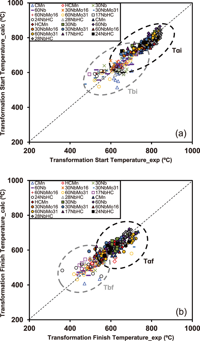
In Fig. 1, experimental and calculated transformation start and finish temperatures are presented. Figure 1(a) corresponds to ferritic (Tαi) and bainitic (Tbi) start temperatures, and Fig. 1(b) shows transformation finish temperatures (Tαf and Tbf). A reasonable prediction is achieved for the transformation start temperatures in both stability regions, especially for polygonal phases (low cooling rates and high transformation temperatures). Although a slightly higher dispersion is detected in bainitic transformation temperatures (see Tbi and Tbf in Figs. 1(a) and 1(b), respectively), the proposed model is able to reasonably estimate transformation temperatures in a wide range of cooling conditions.
Apart from ferritic and bainitic transformation stability regions, the microstructures formed at high cooling rates also present a certain fraction of martensite in conjunction with bainite. A small amount of experimental data concerning pure martensitic transformation temperatures is available in the applied cycles due to the low carbon content of most of the steels studied, and for that reason there is not a considerable amount of martensite in the samples studied. The regression analysis does not provide accurate results when the amount of data is not big enough. Therefore, the empirical equation proposed by Andrews16) in Eq. (8) was used to estimate the martensitic transformation start temperature (Ms) for the construction of the CCT diagrams.
|
Ms=539-423(%C)-30.4(%Mn)-17.7(%Ni)
-12.1(%Cr)-7.5(%Mo)
| (8) |
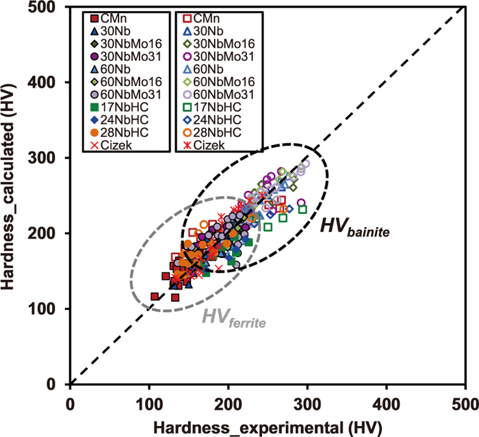
In addition to the transformation temperatures, in order to evaluate the influence of different parameters on mechanical properties, bulk Vickers hardness measurements were taken for each specimen. From these results, equations able to estimate hardness values for both ferritic and bainitic microstructures were derived. Similar to what was considered for transformation temperatures, the regression parameters are chemical composition (%C, %Mn, %Nb and %Mo, in wt%), retained strain in austenite (εacc), average austenite grain size (Dγ, in μm), and cooling rate (CR in °C/s). For hardness prediction a carbon equivalent (CEq) term was calculated based on the Düren’s formula17) for low carbon steels (CEq = C+Mn/16, in wt%). The resulting equations for ferrite and bainite hardness are shown in Eqs. (9) and (10). The adjusted coefficient of determinations are R2adj = 0.71 and 0.69, respectively.
By increasing the microalloying content or carbon level, the formation of bainitic microstructures is more likely, resulting in an increase in hardness. This trend is reflected by the positive sign of the coefficients related to the terms %C, %Mn, %Nb and %Mo. Concerning the accumulated strain (εacc), the proposed equation shows a negative coefficient. The application of deformation in the non-recrystallization region can have different hardness-related effects. On one hand, the accumulation of deformation in austenite promotes the acceleration of transformation, leading to a major presence of ferritic phases that are characterized by lower hardness values. This effect is counterbalanced by the formation of finer ferrite microstructures from pancaked austenite, which provides improved mechanical properties. The competition of these phenomena leads to a small negative coefficient with regard to deformation (εacc). In reference to the term ln(Dγ), increasing the austenite grain size significantly delays the austenite-to-ferrite transformation due to a decrease in the available nucleation site density (less specific grain boundary area (SV)). Coarser austenite unit sizes favor the formation of low temperature microstructures with higher hardness values. Bigger austenite grain sizes cause the stability regions to shift to lower transformation temperatures, as indicated in the proposed relations concerning transformation temperatures (Eqs. (4), (5), (6), (7)). Similarly, it is well known that higher cooling rates cause the lowering of transformation start temperatures, promoting the formation of non-polygonal phases and finer microstructures. The latter transformation products are known to contribute to increased strength, through both small effective grain size and higher dislocation densities.
|
H
V
ferrite
=9.45+739.43(
%C+
%Mn
16
)
+578.42(%Nb)
+44.14(%Mo)-3.19ε+12.40ln(Dγ)-45.90exp(-1.2CR)
| (9) |
|
H
V
bainite
=9.35+994.52(
%C+
%Mn
16
)
+478.05(%Nb)
+74.19(%Mo)-16.74ε+19.17ln(Dγ)-62.75exp(-0.03CR)
| (10) |
In Fig. 2, the hardness values predicted by Eqs. (9) and (10) are compared to experimental values. In this case the hardness values reported by Cizek et al.13) for a Nb microalloyed steel (steel A, 0.046%C-0.212%Si-1.64%Mn-0.045%Mo-0.029%Nb-0.015%Ti) and a Nb–Mo microalloyed steel (steel B, 0.043%C-0.21%Si-1.67%Mn-0.26%Mo-0.022%Nb-0.016%Ti) are also included in the figure in terms of model validation. These steels were submitted to two thermomechanical cycles designed to produce different austenite conditions: non-deformed austenite and deformed austenite. Cizek et al. quantified an austenite grain size of approximately 40 μm in both compositions. The equation predicts reasonably well the hardness values for different chemical compositions, austenite conditions and cooling rates.
3.1.3. Ferrite Unit Size
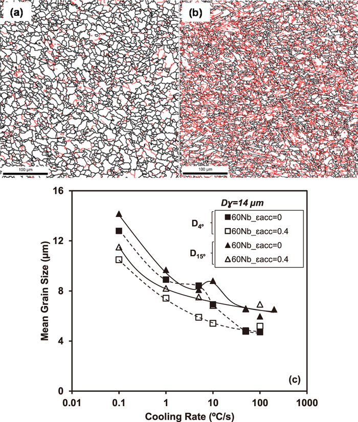
Ferrite unit size prediction is another crucial feature for connecting microstructure and mechanical properties. When non-polygonal microstructures are formed, the EBSD technique is a suitable tool for quantifying mean unit crystallographic sizes. As previously mentioned, 4° and 15° misorientation crystallographic unit sizes were measured using the EBSD technique. Figures 3(a) and 3(b) show boundary maps for the 60 Nb steel with ferritic and bainitic structures, respectively formed at different cooling rates. A higher fraction of low angle boundaries is observed in the bainitic structure (Fig. 3(b)) formed by a combination of quasipolygonal ferrite and granular ferrite. Figure 3(c) shows the dependence of the low and high angle boundary unit sizes on the cooling rate based on the EBSD measurements. Similar trends are observed for all the steels.3)
For the prediction of the ferrite grain size the interaction between the different variables that affect this microstructural parameter must be taken into account. As observed by Bengochea et al.18) the effect of reducing the austenite grain size on refining the ferrite decreases with increasing the accumulated strain. Similarly, the additional refinement produced by increasing the cooling rate weakens as the retained strain increases. This means that a simple linear model would not be appropriated for grain size prediction since interactions are not considered. In the literature different expressions have been proposed. In the present study the following types of equations, Eq. (11) by Sellars and Beynon19) and Eq. (12) by Umemoto,8) have been investigated:
|
D
α
=(
1-a⋅
ε
acc
b
)
⋅(
c
1
+
c
2
⋅
(CR)
p
+
c
3
⋅(1-exp(-0.015⋅
D
γ
))
)
| (11) |
|
D
α
=K⋅
(
D
γ
)
m
⋅
(CR)
p
| (12) |
Equation (12) was developed for recrystallized austenite microstructures and in order to include deformed austenite microstructures, the approach of Lacroix et al.20) was applied and an effective grain size was introduced, i.e.
D
eff
γ
= Dγ · exp(−εacc) (see Eq. (3)). It should be noted that although above equations were derived for microstructures made up primarily of polygonal ferrite, in the present study they have been successfully applied for non-polygonal and bainitic microstructures characterized by EBSD (Fig. 3). A fairly good fit of present results was obtained with both type of equations, although the highest correlation coefficients were achieved with the equation type proposed by Umemoto and modified by the Lacroix´s approach, therefore this was finally adopted. The relationships derived for predicting the mean crystallographic unit sizes, considering low (4°) and high (15°) angle misorientation criteria, are shown in Eqs. (13) and (14), respectively. The variables taken into account in the model are chemical composition (%Nb and %Mo, in wt%), which are included in the constant, austenite grain size (Dγ, in μm), retained strain (εacc) and cooling rate (CR, in °C/s). The adjusted coefficients of determination for both equations are R2adj = 0.91 and 0.93, for the 4° and 15° criteria, respectively, showing a fairly good agreement between the calculated and experimental results.
|
D
mean
(4°,in μm)=(
3.5-12.66(%Nb)-0.93(%Mo)
)
⋅
(
D
γ
exp(-
ε
acc
)
)
0.32
⋅
(CR)
-0.11
| (13) |
|
D
mean
(15°,in μm)=(
2.69-1.83(%Nb)-0.001(%Mo)
)
⋅
(
D
γ
exp(-
ε
acc
)
)
0.41
⋅
(CR)
-0.11
| (14) |
Equations (13) and (14) show that the coefficients corresponding to the chemical composition are negative, which is in agreement with previously reported effects of alloying elements in solution. It is well known that the addition of elements such as Nb and Mo promotes a shift to lower transformation start temperatures in the CCT diagrams, and thus enhancing the formation of finer and more bainitic microstructures.3) Furthermore, the above-mentioned refinement associated with lower austenite grain sizes and higher retained strains is reflected. Similar trends are also reported in the research carried out by Bengochea et al.21) and van Leeuwen et al.,22) where the influence of the prior austenite grain size, the retained strain and the cooling rate on the final ferrite microstructure was analyzed. Those authors suggested that the reduction of austenite grain size and the increase of retained strain provide a higher density of nucleation sites, and therefore a refinement of the resultant microstructure. Coarser austenite grain sizes involve the formation of larger ferrite mean unit sizes for both misorientation criteria.
In terms of the cooling rate (CR), the mean unit sizes decrease as the cooling rate increases. Sellars and Beynon,19) in the case of microstructures made up primarily of ferrite, found a relationship between the ferrite grain size (Dα) and the cooling rate of CR−0.5. In the present case, the regression analysis resulted in a relationship of CR−0.11, denoting a lower effect of the cooling rate on grain size. This is probably related to the fact that in the present results a wider range of microstructures is taken into account, including non-polygonal ferrite and bainite, which form at higher cooling rates than polygonal ferrite, resulting in a weaker effect of this parameter on grain size, as previously observed by Olasolo et al.14)
Calculated mean unit sizes versus experimental unit sizes measured by means of EBSD are plotted in Fig. 4. Figures 4(a) and 4(b) correspond to low and high angle misorientation criteria, respectively. The solid symbols are related to coarse prior austenite grain sizes in the 84–125 μm range,2) whereas the open symbols refer to fine austenite grain sizes, between 12 and 19 μm.3) Figure 4 shows higher dispersion when the microstructures are composed of coarser crystallographic unit sizes. These deviations can be attributed to the formation of coarse bainitic units that deviate from the general trend as reported by Isasti et al.3) and Furuhara et al.23)
3.2. Relative Weight of the Metallurgical Parameters
The comprehension of the relative contribution of the different metallurgical parameters involved in the prediction equations proposed in the current paper is not straightforward. For a better understanding of which parameters have a key role on each property, the radar plot in Fig. 5 gathers the relative contribution of each parameter in values such as the initial transformation temperatures, hardness and mean grain sizes. Based on Eqs. (4), (5), (9), (10), (13) and (14), the variation needed for each individual addend to modify by 1% the predicted magnitude is evaluated. This approach was followed due to the different magnitudes plotted in Fig. 5, such as in the temperatures (°C) (Fig. 5(a)), hardness values (Fig. 5(b)) and grain sizes (μm) (Fig. 5(c)), as well as in the input parameters such as chemical compositions (wt%), austenite grain sizes (μm) and retained strain. Once the variation needed for each input variable to modify in 10% the predicting magnitude is calculated, a value of 1 is given to the most influencing factor and the relative weight of the remaining factors calculated. Therefore, if for a given magnitude, one factor has a 0.2 value in the plot, a variation 5 times bigger than the factor with the value of 1 should be applied to reach an equivalent impact.

For example, if the Dmean(4°) parameter is analyzed in detail (Eq. (13) and Fig. 5(c)), the following calculations result. For the given input parameters of 0.05%C, 0.03%Nb, 0.16%Mo, 1%Mn, εacc = 0.4, Dγ = 20 μm and CR = 1°C/s, a value of Dmean(4°) = 6.8 μm is predicted. Now, the variation of each parameter needed to modify, for example, 10% the predicted magnitude is calculated. Niobium has to be increased up to 0.054%Nb (an 80% increment from the initial 0.03% value), Molybdenum up to 0.48% (an increment of 200%), the accumulated strain to 0.73 (an increase of 82.5%) and the prior austenite grain size has to decrease to 14.4 μm (a decrease of 29%). All these variations are equivalent in their impact to the Dmean(4°) value, resulting in a variation of 10% from the initial 6.8 μm to 6.12 μm. Therefore, the most influencing factor is the prior austenite grain size, since with the lowest variation affects the most the predicted magnitude. So, if a weighting factor of 1 is given to Dγ, and the other factors are corrected by this relative weighting, a relative impact of 0.36 (29/80) is calculated for Nb, 0.145 (29/200) for Mo and 0.35 (29/82.5) for εacc. These values are the ones plotted in Fig. 5(c). Similar calculations were made by all the magnitudes calculated.
From a general point of view, Fig. 5 shows that prior austenite grain size (Dγ) is the most influencing factor for the ferrite start transformation temperature and both low and high angle boundary grain sizes, carbon content for bainite start temperature and Mn content for hardness values. Small variations in these input factors would strongly affect the predicted magnitudes. Ferrite transformation start temperature is also importantly affected by accumulated strain and molybdenum content. Hardness levels (Fig. 5(b)) are strongly controlled by C and Mn levels, and in a lower degree by Nb level and prior austenite grain size.
For the mean grain sizes plotted in Fig. 5(c), both prior grain size and accumulated strain have equivalent influence on low and high angle boundary units. However, chemical composition only affects low angle boundary structure, while for high angle grains the direct effect of Nb and Mo is negligible. This consideration doesn’t mean that the predicted magnitudes are not affected by changes in the chemical composition, as it is well stated that Nb and Mo microalloying exert an important control over austenite evolution during hot rolling. Therefore, indirectly, these elements are promoting a ferrite grain size refinement through austenite pancaking, i.e. strain accumulation. Similarly, the large effect of Nb on hardness arises from the above mentioned ferrite refinement effect to which the possible contribution of precipitation hardening of Nb carbonitrides, which is enhanced by increasing Nb content, would be added.
3.3. CCT Diagram Modeling
The experimental and predicted CCT diagrams corresponding to different chemical compositions, austenite grain size and retained strain conditions are shown in Figs. 6, 7, 8, 9. The predicted diagrams are indicated by solid lines, and they were obtained by using the equations corresponding to transformation start and finish temperatures proposed in Eqs. (4), (5), (6), (7). Experimental points are indicated by solid symbols. Measured and predicted hardness values are also included. In some cases, the ferritic and bainitic transformation start temperature curves intersect. This intersection is considered to be the limit of both stability regions. When the curves do not intersect, the validity range of each equation needs to be taken into account. Cooling rates between 0.1 and 5°C/s are considered to be the lower and upper limits for the ferritic region. For higher cooling rates, the equations developed for the bainitic region are applied.
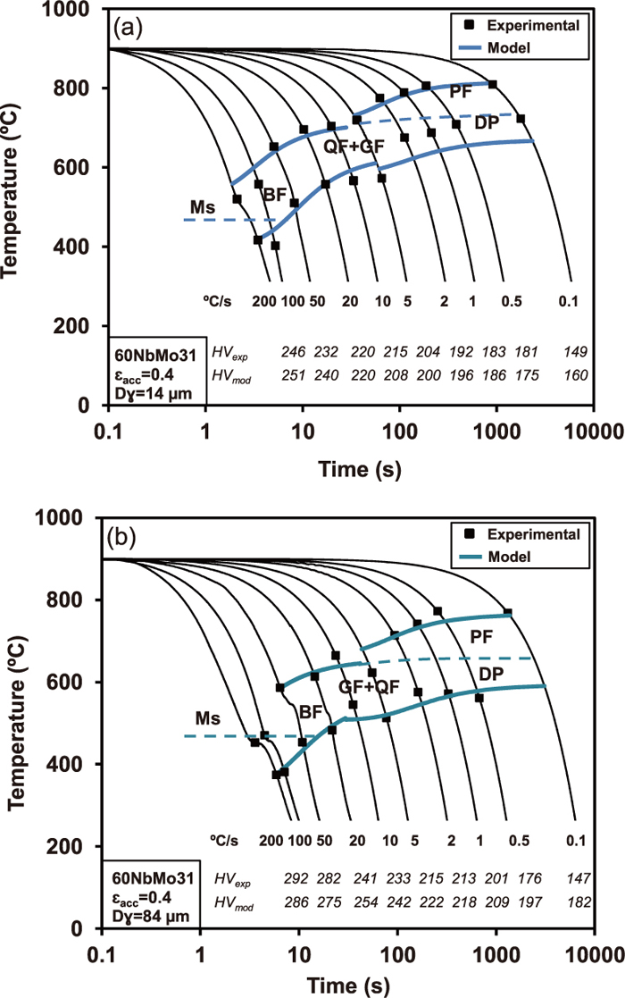
In order to evaluate the effect of prior austenite grain size on transformation behavior, the CCT diagrams calculated for the 60NbMo31 steel for different austenite grain sizes but similar retained strain are represented in Figs. 6(a) and 6(b), for fine and coarse austenite grain sizes, respectively. The model predicts CCT diagrams accurately for the ferritic and bainitic transformation regions and the effect of different austenite grain sizes prior to transformation. Furthermore, Fig. 6(b) exhibits good agreement between the predictions of the empirical equation reported by Andrews16) and experimental martensitic transformation start temperatures.
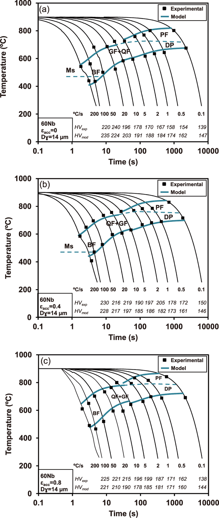
CCT diagrams obtained for the 60Nb steel and transformed from different austenite conditions are shown in Fig. 7. Figure 7(a) is for recrystallized austenite, while Figs. 7(b) and 7(c) present the stability regions corresponding to deformed austenite and accumulated strain levels of 0.4 and 0.8. Figure 7(a) shows that the equations reproduce the effect of retained strain fairly well when deformation varies from 0 to 0.8.
Looking at the effect of chemical composition, the stability regions related to different steels (CMn, 30NbMo0 and 30NbMo31) are shown in Fig. 8. A fairly good prediction of the CCT diagrams is observed by varying the chemical composition. In the CMn steel, quite good agreement between experimental and model temperatures (Fig. 8(a)) is achieved for the entire range of investigated cooling rates. However, in the microalloyed steels (30NbMo0 and 30NbMo31, in Figs. 8(b) and 8(c), respectively) the model presents a slight deviation of the bainitic start and finish transformation temperatures leading to higher predicted transformation temperatures (Tbs and Tbf). Even though the equations related to the ferritic region appropriately reproduce transformation temperatures, the model predicts slightly higher transformation temperatures when non-polygonal phases dominate the resultant microstructures.
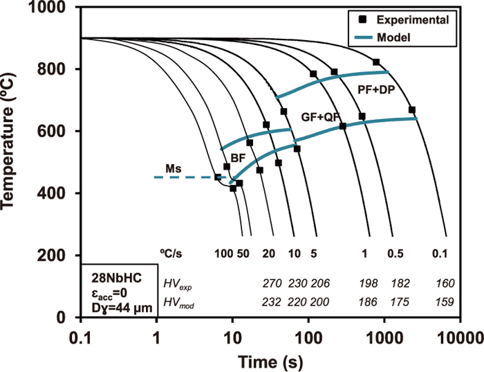
The CCT diagram corresponding to the 28NbHC steel, which contains a higher carbon (0.09%C) and lower manganese (0.99%Mn) levels, is shown in Fig. 9 in order to evaluate the potential of carbon to shift the stability regions. As detailed in Eqs. (4) and (5), the effect of carbon is only considered in the bainite start temperature but not in the ferrite start. Figure 9 shows that even if the ferrite start temperature curve is correctly predicted, a noticeable deviation is observed for the bainite start and finish transformation temperatures. This effect can be related to the relatively limited amount of data available for the steels containing a higher amount of carbon, which could restrict the accuracy of the predictions in this range.
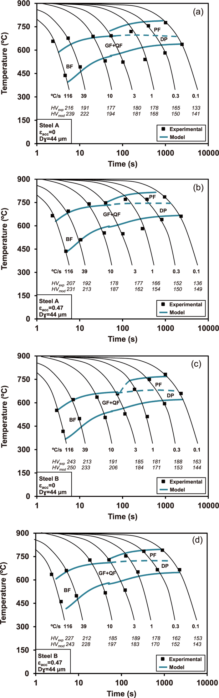
In order to extrapolate the ability of the model to reproduce CCT diagrams for external experimental data, various CCT diagrams reported in the literature were reproduced. As for hardness measurements, the experimental data reported by Cizek et al.13) were used for that purpose (previously mentioned Nb and Nb-Mo microalloyed steels A and B. Steel B is also microalloyed with Ti). For the case of steel B, the main effect of Ti during thermomechanical treatments of steels is limited to grain growth control of austenite during the interstand times. Titanium would affect indirectly phase transformations through austenite refinement but as the austenite grain size is an input for the proposed equations there is no need to include Ti effect explicitly in the regression equations. Figure 10 illustrates the comparison between experimental data reported by Cizek et al.13) and the results obtained from the present model. Figures 10(a) and 10(b) correspond to the Nb microalloyed steel transformed from non-deformed (εacc = 0) and deformed (εacc = 0.47) austenite, respectively, while Figs. 10(c) and 10(d) present the Nb-Mo microalloyed steel results at both austenite conditions. The proposed equations offer a good fit for the start and finish transformation temperatures, and therefore a reasonable prediction of the CCT diagrams for both steels. In particular, in the case of deformed austenite the stability regions of the different phases are fairly well reproduced.
;%0A%09%09%09newWindow.document.open();%0A%09%09%09newWindow.document.write('<img src=%22./Graphics/55_1963_tbl_1.jpg%22>');%0A%09%09%09newWindow.document.close();%0A%09%09)