Abstract
A thermodynamic model coupling microsegregation and inclusion formation using one ChemSage datafile is proposed. The thermodynamic equilibrium is calculated using ChemApp to determine the liquidus temperature, solute partition coefficients at the solidification interface and inclusion formation in the residual liquid. During the calculations, solute enrichment is predicted using Ohnaka’s model. The logarithm of the coupling microsegregation and inclusion formation is tested through an overall mass balance. With the proposed model, inclusion formation is predicted for the case of medium carbon steels alloyed with titanium and aluminum. The predicted types and compositions of inclusions agree well with the experimental results. Based on the predictions and measurements, the inclusion behavior during solidification is discussed.
1. Introduction
Massive oxide and sulfide inclusions can negatively affect the process ability of steel as well as the technological properties of steel products. Hence, many efforts have been made during the last few decades to optimize steelmaking technologies to achieve a lower amount of non-metallic inclusions in the steel matrix and to control their size and chemical composition. This evolution led to so-called “clean steel production”.1)
In contrast, fine dispersed oxides may act as inoculants for the heterogeneous nucleation of complex inclusions. These inclusions may finally be active for grain refinement during solidification2,3) and for the control of microstructure formation in the solid state4,5,6) just to name two examples. The adjustment of oxides to act as inoculants was recognized in the 1980s7,8) and termed “oxide metallurgy”.
The first computer programs for simulating the compositional changes of inclusions during solidification also originate from the 1980s: Yamada et al.9) coupled the Clyne-Kurz microsegregation model with thermodynamics for the formation of oxide phases and CaS in liquid steel. The resultant model enabled the estimation of the composition and the amount of complex oxide and sulfide inclusions during solidification of a Ca-treated Al-deoxidized steel. Based on a similar approach, Wintz et al.10,11) analyzed the formation of (Mn, Fe)S in steel with a varying Mn/S-ratio and the formation of complex oxide inclusions in semi-killed steels and validated the results using experiments and microprobe analysis. Choudary and Ghosh12) predicted the interdendritic enrichment using the Clyne-Kurz-model and calculated the phase stability of the oxide and sulfide phases using the commercial software.13) Nurmi et al.14) coupled the IDS15) solidification model for steel with the -thermodynamic library16) and then calculated the evolution of inclusions during secondary metallurgical treatment and subsequent casting and solidification. For a broad field of examples, the calculated results correspond well to the measurements; this performance certainly explains the frequent use and popularity of these models.9,10,11,12,14)
The present work addresses the approach that is schematically depicted in Fig. 1. Heat and mass transfer at the macroscopic scale, enrichment of elements, and the kinetics of the precipitation of phases at the microscopic scale are solved in a FORTRAN program. For each calculation step, the composition is transferred to ChemApp based on the thermodynamics of the FactSage, and the program libraries are used to determine the liquidus temperature, equilibrium partition coefficients at the solid-liquid interface, and volume fraction of the stable phases. Currently, the model is further developed to consider heterogeneous nucleation and the subsequent growth of particles in the future and thus to predict not only the chemical composition and volume fraction of particles but also their size distribution. The just- described approach offers the following specific characteristics:

• A numerical solution of Ohnaka’s model17) for columnar dendrite geometry was selected for microsegregation calculations.18) Diffusion coefficients are temperature dependent and the equilibrium partition coefficients are calculated based on thermodynamic equilibrium for every time step.
• The commercial databases provide not only the thermodynamic data for oxide and sulfide inclusions (as discussed in this paper) but also for primary carbides or nitrides (which are of highest interest in the solidification of high alloyed steels). The databases used are both commercial ones and self-adjusted databases.19)
• Trapping of inclusions by the solidification interface was treated in a simple manner as suggested by Yamada et al.9) The logarithm of coupling microsegregation and inclusion formation was tested through an overall mass balance. The detailed tests of the microsegregation model including ‘communication’ of the FORTRAN source code with the thermodynamic datafile, have been reported in Ref. 18).
In this paper, the changes of inclusion compositions, types and amounts for three selected steels were predicted applying the coupled model. The calculations were compared with the experimental results. Finally, the behavior of non-metallic inclusions during the solidification process was discussed based on the predictions and measurements.
2. Model Description
The following thermodynamic equilibrium calculations were performed using ChemApp and the ChemSage datafile. The datafile was created from FactSage 7.0 based on FSstel and FToxid. ChemApp is an interface software developed by GTT Technologies, Herzogenrath, Germany. This interfacial software can be linked to a source code written in FORTRAN, C/C++, Visual Basic® and Borland Delphi®. In this case, FORTRAN was applied as the programming language to solve the kinetics of solidification (cooling, microsegregation, nucleation and growth and entrapment of inclusions). Microsoft Visual Studio 2013 was used as the main frame provider and modern compiler.
2.1. Microsegregation Calculation
For considering the changes of the partition and diffusion coefficients, Ohnaka’s model was integrated into Eq. (1). The local partition coefficients and diffusion coefficients were calculated at each solidification step; however, within the increase of the solid fraction by Δfs, they were assumed to be constants.
|
C
L
+
=
C
L
{
1-Γ⋅
f
s
1-Γ⋅(
f
s
+Δ
f
s
)
}
1-k
Γ
, with Γ=1-
4αk
1+4α
| (1) |
|
α=
4
D
s
t
f
(
λ
2
)
2
| (2) |
In Eq. (1) fs represents the solid fraction; CL and
C
L
+
are the concentrations of the solutes in the residual liquid at solid fractions of fs and fs+Δfs, respectively; k is the equilibrium partition coefficient between the solid and the liquid; α is the back diffusion coefficient, which can be calculated using Eq. (2); Ds is the solute diffusion coefficient in the solid; tf is the local solidification time; and λ2 is the secondary dendrite arm spacing.
In the applied model, the temperatures at the solidification interface and partition coefficients (k) were calculated using thermodynamic databases. At each solidification step, for a multicomponent system, the phase transformation point from liquid to solid was detected after the activity of δ-ferrite or austenite achieved a value of 1. Next, the concentration of solutes in both liquid and solid and the temperature was determined. The diffusion coefficients (Ds) applied in the calculations are listed in Table 1. The partition and diffusion coefficients used for the calculations are the average values between the respective values at the current and the former time step. The temperatures were updated in a loop until the difference between two adjacent values was less than 10−3 K.
Table 1. Diffusion coefficients of solutes.
9,20,21)| Elements | Dδ (m2s−1) | Dγ (m2s−1) |
|---|
| C | 0.0127Exp (−81301/RT) | 0.0761Exp (−134429/RT) |
| Si | 8.0Exp (−248710/RT) | 0.3Exp (−251218/RT) |
| Mn | 0.76Exp (−116935/RT) | 0.055Exp (−249128/RT) |
| P | 2.9Exp (−229900/RT) | 0.01Exp (−182666/RT) |
| S | 4.56Exp (−214434/RT) | 2.4Exp (−212232/RT) |
| O | 0.0371Exp (−96349/RT) | 5.75Exp (−168454/RT) |
| Al | 5.9Exp (−241186/RT) | 5.15Exp (−245800/RT) |
| Ti | 3.15Exp (−247693/RT) | 0.15Exp (−251000/RT) |
| Ca | 0.76Exp (−224430/RT) | 0.055Exp (−249366/RT) |
R: 8.314 J/(mol·K); T: temperature in Kelvin.
The secondary dendrite arm spacing was estimated using Eq. (3); thus, the estimation considered the influence of the local solidification time and initial carbon content.22) Initially, the local solidification time is estimated. After determining the first solution for the solidus temperature, the local solidification time is calculated according to Eq. (4). In Eqs. (3) and (4), λ2 (μm) denotes the secondary dendrite arm spacing, C0 is the initial concentration of carbon in mass percent, tf (s) is the local solidification time, Rc (K/s) is the cooling rate, and TL and TS (K) are the liquidus and solidus temperatures, respectively. This process was repeated until the difference between two adjacent local solidification times was less than 10−4 seconds.
|
λ
2
=(
27.3-13.1
C
0
1
3
)
t
f
1
3
| (3) |
In addition, the peritectic reaction was realized in a simple manner similar to other analytical models: if it detects that the solid phase at the solidification interface will change from δ-ferrite to austenite, then the partition and diffusion coefficients of austenite were applied. Further information regarding the microsegregation model was reported in former study.18)
2.2. Inclusion Formation
The stability of non-metallic phases (here oxides and sulfides) in the residual liquid was calculated based on thermodynamic databases. Note that in the present model, inclusions formed before solidification were also considered. During the calculations, both stoichiometric and solution phases can be accounted. The compositions and the components of the solution phases are available. Figure 2 explains the modeling of pre-existing inclusions during solidification. It was assumed that the pre-existing inclusions were distributed evenly in the residual liquid above the liquidus temperature. After the start of solidification, the formed inclusions were partly trapped by the solidifying interface. The amount of trapped inclusions was calculated according to Eq. (5).9) These trapped inclusions in solid steel are assumed to be inert in the ongoing calculation process. Considering microsegregation, the residual inclusions may grow or resolve and new inclusions can precipitate. After balancing the masses of the elements, the concentrations in the liquid were used for the microsegregation calculation in the next step. The flow chart of the coupled model is shown in Fig. 3.
|
Amount
trapped
=
Amount
in liquid
* Δ
f
s
/(
1-
f
s
)
| (5) |
In this section, the algorithm of the fully coupled microsegregation and inclusion formation model was tested according to an overall mass balance for steel A with the composition listed in Table 2. When setting the back diffusion coefficient (α) in Ohnaka’s model to zero, Eq. (1) becomes Eq. (6), which is the analytical equation of Scheil’s model.23) To simplify the calculation of the solute amount in solid steel, Eq. (6) was applied for the microsegregation calculation in this test. It was assumed that solidification was completed at a solid fraction of 0.95. The results are shown in Fig. 4.
|
C
L
+
=
C
L
{
1-(
f
s
+Δ
f
s
)
1-
f
s
}
k-1
| (6) |
Table 2. Chemical compositions of steels (mass%).
| Steels | C | Si | Mn | S | P | Al | Ca | Ti | O | N |
|---|
| A | 0.2 | 0.05 | 1.00 | 0.0060 | 0.0010 | 0.0300 | 0.0020 | – | 0.0020 | – |
| B | 0.23 | 0.02 | 1.48 | 0.0074 | 0.0040 | 0.0051 | – | 0.0500 | 0.0050 | – |
| C | 0.24 | 1.80 | 1.91 | 0.0060 | 0.0040 | 0.0040 | – | 0.0310 | 0.0029 | 0.0039 |
| D | 0.26 | 1.84 | 2.07 | 0.0050 | 0.0040 | 0.0040 | – | – | 0.0040 | 0.0022 |

Figure 4 describes the changes of inclusions during the solidification process. ASlag and CaS are found to be stable at the liquidus temperature. Here ASlag is a solution phase whose components are mainly Al2O3, CaO, Al2S3, CaS and SiO2. At the solid fraction of 0.1, the ASlag phase transforms into CaS and CaO·Al2O3. Next, with the stronger enrichment of solutes and decreasing temperature, CaO·Al2O3 becomes unstable and becomes CaO·6Al2O3 at solid fraction of 0.7. During the changing of inclusions and enriching of solutes, the overall mass balances of all of the solutes were calculated. Compared with the input amount, a maximum relative difference of 0.05% was found for oxygen, whereas for the other elements, the maximum relative difference remains below 0.02%. With respect to the initial oxygen content in steel A of 0.002%, the inconsistency in the mass balance amounts to only 10−2 ppm. The observed differences can be primarily explained as the sum of the residuals in the iteration steps and by the abrupt increase of the partition coefficient during the peritectic reaction. With respect to the five involved inclusion types and continuous changes of their mass fraction as well as the change in partition coefficients due to the peritectic reaction the inconsistency in the mass balance is apparently in an acceptable range.
3. Experiments
3.1. Melting Experiments
Steels B, C and D were produced on a laboratory scale. To achieve specific inclusion types and a possibly homogeneous distribution of non-metallic inclusions in the steel matrix, an easily controllable small-scale furnace is used for all experiments. The Tammann type furnace (Ruhrstrat HRTK 32 Sond.) is a high-temperature electric resistance furnace that can be heated to 1700°C. Due to the carbon heating tubes inside the furnace and their reaction with the residual oxygen, the final oxygen content in the furnace vessel is extremely low (0.001 ppm). The schematic experimental setup before starting the experiment is schematically shown in Fig. 5. All experiments are conducted under an inert gas atmosphere. The experimental procedure consists of the following main steps:

• Approximately 100 g of unalloyed steel (0.004 wt% C, 0.066 wt% Mn and 0.006 wt% S, rest Fe) is placed in an Al2O3 crucible together with an oxygen-rich pre-melt (0.001 wt% C, 0.075 wt% Mn and 0.009 wt% S, 0.175 wt% O, remainder Fe). Due to the thermal and mechanical stresses during the experiment, the Al2O3 crucible is also placed into a graphite crucible. A Mo-wire which is used to remove the crucible from the furnace is fixed at the top of the graphite crucible (“elevator system”).
• The crucible with the raw materials is heated to 1600°C at a rate of 10 K/min, resulting in a melt that has a defined oxygen content of approximately 300 ppm. After 6 min the melt is stirred with an Al2O3 bar and C, Mn and Si are added according to the desired final chemical composition. This process also involves a decrease in the oxygen content and the formation of non-metallic inclusions.
• After another 8 min, the melt is stirred again and FeTi75 is added (only for steels B and C), which again provokes the formation of new inclusions and the modification of pre-existing inclusions. FeTi75 means the Fe-75wt% Ti alloy. After holding for another 5 min at 1600°C and a final stirring, the crucible is quickly removed from the heating zone of the furnace by the use of the Mo-wire and then quenched rapidly through casting into a mold to prevent distinct inclusion flotation during solidification.
The total experimental time of 19 min at the experimental temperature was the same for all experiments. The only difference consisted of the addition of FeTi75 alloy for steels B and C, whereas for steel D, no FeTi75 was alloyed. Note that Al was not added directly in any of the experiments. The presence of Al in the melt and consequently in the inclusion is the result of reactions with the crucible material used as well as the bar for stirring the melt.
The final cast sample has a spherical shape with a diameter of 50 mm. In the first step, the chemical composition of the sample was determined using classical optical emission spectrometry. The sample was then cut into equal halves: one part was used for inclusion analyses; the other part was used to produce small slices (cut from the part) for the determination of the oxygen and nitrogen contents via LECO analyses. The final chemical compositions of the examined samples are listed in Table 2. Further details regarding the Tammann Furnace experiments can be found elsewhere.6,24)
3.2. Inclusion Characterization
Automated SEM/EDS analyses using an FEI Quanta 200 MK2 scanning electron microscope (SEM), equipped with an energy dispersive X-ray spectrometer (EDS) system from Oxford Instruments were performed to characterize the inclusion number, size and type in the produced samples of steels B, C and D. The latter method is currently state-of-the-art concerning the determination of steel cleanness in steels.25,26,27,28) Based on the automated SEM/EDS analysis, inclusions are detected due to the material contrast differences in the backscattered electron (BSE) image. Usually, non-metallic inclusions are displayed as darker compared to the steel matrix. The automated analyses are performed at an accelerating voltage of 15 kV and are limited to a minimum particle size of 1.1 μm ECD (Equivalent Circle Diameter). Principally a measurement area of 100 mm2 is defined on the sample surface. However, because samples that are in the as-cast condition are not deformed after the melting experiment, the analysis is limited to a maximum of 6000 particles on the defined area to avoid an extensive measurement time caused by the presence of micropores. The inclusion distribution over the analyzed sample area was found to be very homogeneous, and in all cases, more than 90 mm2 was analyzed.
4. Results
4.1. Calculation Results
The three steels B, C and D were calculated using the proposed coupled model. The cooling rate was assumed to be 10 K/s for all three steels considered. Note that the exact cooling rates of the aforementioned experiments are difficult to define. For this reason, taking Steel B as an example, the influence of the cooling rate on the inclusion formation during solidification will also be discussed in this section.
(1) Steel B
Figure 6(a) shows the calculated inclusion formation behavior at a cooling rate of 10 K/s. Four types of inclusions are predicted: ASlag, MnS, Al2O3 and Ti3O5. The components of the solution phase -of ASlag- are mainly Al2O3, MnO, Ti2O3 and TiO2. The exact compositions of ASlag will be discussed in a later stage. The primary inclusions before solidification are ASlag and Al2O3. Next, ASlag increases and Al2O3 decreases at a small scale until reaching a solid fraction of 0.1. At the solid fraction of 0.1, ASlag becomes unstable and then decomposes into Ti3O5 and Al2O3, leading to the sharp increases of Ti3O5 and Al2O3. However, note that these sudden changes are not reasonable when considering the kinetic processes. In the subsequent process, Ti3O5 is more stable than Al2O3 in the following process and precipitates with the consumption of Al2O3. MnS forms at the late stage of solidification due to the microsegegation of sulfur (S) and manganese (Mn). Finally, in addition to Ti3O5 and MnS, small amounts of ASlag and Al2O3 still exist due to trapping by solid steel.

To investigate the influence of the cooling rate on the inclusion formation thermodynamics, another calculation is performed for Steel B applying a cooling rate of 0.1 K/s. The calculation result is shown in Fig. 6(b). Compared with the result assuming a cooling rate of 10 K/s, as shown in Fig. 6(a), the inclusion types are the same when including Ti3O5, MnS, ASlag and Al2O3, and their evolution processes are also the same. The amount of oxides calculated with different cooling rates is similar. The amount of MnS under a cooling rate of 10 K/s is approximately twice that of the cooling rate of 0.1 K/s because of the higher enrichment of S and Mn. The higher cooling rate also yields to a lower solidus temperature because of stronger microsegregation. Therefore, a reasonable cooling rate must be selected especially for the prediction of microsegregation-induced precipitations (such as MnS), whereas the influence of the cooling rate on the formation of oxides can practically be neglected for the present case.
(2) Steel C
Figure 7 displays the inclusion changes that occur during the solidification of Steel C. Five types of nonmetallic inclusions are observed: ASlag, MnS, Al2O3, Ti3O5 and Ti(C, N). The ASlag phase is composed of Al2O3, SiO2, MnO, Ti2O3 and TiO2. In addition to ASlag, Ti(C, N) is also a solution phase, in which the amount of carbon (C) increases gradually because of microsegregation. ASlag and Al2O3 already exist in liquid steel. After solidification starts, the amount of ASlag increases, whereas that of Al2O3 decreases. ASlag transforms into Ti3O5 and Al2O3 at a solid fraction of 0.5. Similar to ASlag in Steel B, the sudden decomposition results in only a small amount of ASlag in the solid steel. Ti3O5 starts to precipitates from this point and the content of Al2O3 continues to decrease. Next, Ti(C, N) forms at a solid fraction of 0.7 due to the microsegregation of titanium (Ti) and nitrogen (N). The enrichments of Mn and S promote the precipitation of MnS after reaching a solid fraction of 0.94. The formation of Ti(C, N) and MnS highlights the importance of microsegregation. Note that the amount of different inclusions from the calculation only offers a basic reference. For an accurate estimation of the absolute contents, the kinetics must be considered.

Figure 8 describes the inclusions formation during solidification of Steel D. ASlag, Al2O3 and MnS compose the inclusions in Steel D. Without Ti addition, Al2O3, SiO2 and MnO are the primary components of the ASlag phase. ASlag and Al2O3 form before solidification. During the solidification process, ASlag gradually increases and Al2O3 decreases. MnS precipitates at the late stage of solidification. Compared with Steels B and C, the types and changes of inclusions are relatively few due to the absence of Ti addition.
4.2. Experimental Results
Figure 9 shows the inclusion types and frequencies of inclusions in the three steels obtained from automated SEM/EDS analyses. For each type of steel, the main inclusion types are listed; inclusion types with a relative frequency of less than 2% were summarized in the class “others”. For Steel B, the predominant inclusion types are (Ti, Al, Mn)xOy, TiOx, MnS and Al2O3-TiOx. The other types are mainly the heterogeneous inclusions of the aforementioned oxides and sulphides; among them, the frequency of (Ti, Al, Mn)xOy and TiOx account for approximately 90%.
In Steel C, (Ti, Al, Si, Mn)xOy , MnS and Ti(C,N) are the main inclusions. Compared with Steel B, the frequencies of oxides are decreased, in agreement with the lower oxygen content in steel C. The enrichments of nitrogen (N) and carbon (C) result in the precipitation of Ti(C,N). Carbonitrides and sulfides are likely to nucleate heterogeneously.
For Steel D, the types of inclusions are significantly different due to the absence of Ti. (Al, Si, Mn)xOy, MnS and oxysulfides are the prevailing types. Similar with Steel C, the microsegregation of solutes contribute to the high frequency of MnS. Hardly any pure Al2O3 was detected in any of the three steels considered.
5. Discussion
In this section, the correspondence of the calculated and experimental results is discussed. The inclusion formation processes in Steels B, C and D were analyzed based on the calculations and measurements.
(1) Steel B
For comparing the measured and predicted types of inclusions, it is important to realize that the model cannot picture heterogeneous nucleation. Consequently, a direct comparison between the measured and calculated inclusions is not approvable for all types. In detail, a comparison between measured and calculated inclusion types leads to the following results:
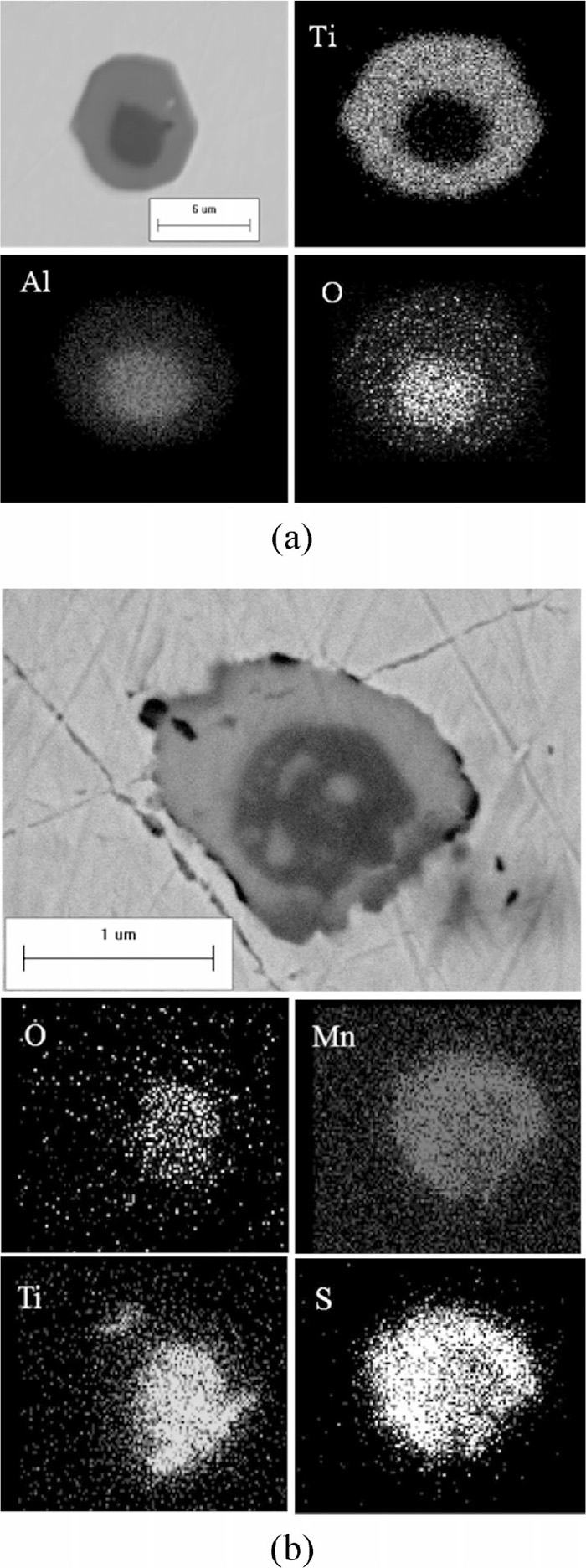
• The solution phase (Ti, Al, Mn)xOy reflects the largest percentage in Steel B. Figure 10 shows the morphology and the corresponding EDS spectrum of the (Ti, Al, Mn)xOy phase. The shape and nature of this inclusion type suggests its liquid occurrence at the processing temperature. As illustrated in Fig. 11, the average composition of this measured phase (measurement of the whole particle) is in very good agreement with the calculated ASlag Phase, which is the predominant phase at low solid fraction in the calculations (see Fig. 6(a)). Thus, a correspondence between the measured and calculated results for this type can be assumed.

• TiOx and MnS are found by both measurement and calculation as shown in Figs. 6(a) and 9. As stated in the literature, Ti3O5 can transform into other titanium oxides in solid steel.29) In addition, a clear distinction between different titanium oxides in the automated measurement results is also difficult to obtain due to unavoidable effects, such as the dependence of the excitation of the inclusions’ surrounding matrix with the size of the inclusions’. Thus, the exact fit of predictions and measurements regarding the stoichiometry of the oxides cannot be expected, although the comparison showed a satisfying accordance.
• Table 3 summarizes the correspondence of the predicted and measured inclusion types in Steel B. The homogeneous inclusions (Types 1, 2, and 3) are in good agreement. For the heterogeneous inclusions Al2O3–TiOx and TiOx–MnS (Types 4 and 5), no direct accordance is found because - as stated before -heterogeneous nucleation is not considered by the presented model. However, the order of inclusion formation can be predicted which indirectly can be used to explain the formation of these inclusion types.
Table 3. Correspondence of the predicted and measured inclusions in Steel B.
| Types | 1 | 2 | 3 | 4 | 5 |
|---|
| Measured | (Ti, Al, Mn)xOy | TiOx | MnS | Al2O3–TiOx | TiOx–MnS |
| Calculated | ASlag | Ti3O5 | MnS | Al2O3 | – |
| Corresponding | Yes | Yes | Yes | Possible | Possible |
Al2O3 is likely to act as a heterogeneous nucleus for TiOx and other oxides, whereas TiOx itself can also act as a potential nucleus for the precipitation of MnS (see Figs. 12(a) and 12(b)). In the automated measured results (Fig. 9), heterogeneous TiOx–MnS (Fig. 12(b)) inclusion is classified into others. Based on the assumptions and explanations above, the following inclusion formation order is proposed: Al2O3, Ti3O5, and MnS. The same order is described by the calculations as shown in Fig. 6(a).
Regarding the inclusion frequencies, from Fig. 9, we can find that the contents of homogeneous inclusions in Steel B occur in the following order according to the measurements: (Al, Ti, Mn)xOy , TiOx, and MnS. For the predictions (Fig. 6(a)), the content decreases from Ti3O5 to MnS and to ASlag. Note that this difference results from the transformation balance between TiOx and ASlag. One possible reason for the discrepancy is that instead of thermodynamically sudden decomposition shown in Fig. 6(a), the (Al, Ti, Mn)xOy (ASlag) could transform into TiOx with low speed. Thus, in solid steel, there is a larger amount of (Al, Ti, Mn)xOy oxide than TiOx.
(2) Steel C
• For studying the correspondence of the inclusion types, it is necessary to define the solution phase (Ti, Al, Si, Mn)xOy. The spherical shape and chemical composition of the solution phase given in Fig. 13 indicate the possibility of corresponding to the ASlag phase. Figure 14 compares the average measured compositions of (Ti, Al, Si, Mn)xOy (measurement of the whole particle) and calculated ASlag. The good agreement illustrates their correspondence.
• Table 4 lists the corresponding inclusion types from the predictions and measurements in Steel C. In addition to the (Ti, Al, Si, Mn)xOy solution phase, TiOx, Al2O3, MnS and Ti(C, N) are also identified in both calculations and experiments. Note that it is difficult to compare the compositions of Ti(C, N) due to the largely changeable nature in the microsegregation process of solutes.
Table 4. Correspondence of the predicted and measured inclusions in Steel C.
| Types | 1 | 2 | 3 | 4 | 5 |
|---|
| Measured | (Ti, Al, Si, Mn)xOy | TiOx | Al2O3 | MnS | Ti(C, N) |
| Calculated | ASlag | Ti3O5 | Al2O3 | MnS | Ti(C, N) |
| Corresponding | Yes | Yes | Yes | Yes | Yes |
Regarding the inclusion formation order, it is clear that various oxides form before MnS and Ti(C, N). MnS and Ti(C, N) precipitate at the late stage of solidification because of segregation. It is also possible for pre-existing (Ti, Al, Si, Mn)xOy to transform into TiOx and Al2O3. However, when considering the transformation kinetics, the occurrence of sudden and complete decomposition appears to be unreasonable.
For the inclusion frequency, the prediction (Fig. 7) shows that the oxides, manganese sulfide and titanium carbonitride share similar frequencies, and the measurement (Fig. 9) displays similar frequencies of to those of the oxides and manganese sulfide as well as a smaller percentage of carbonitrides. For a simple comparison, the applicability of the calculation and experiment is considered to be acceptable. Among the oxides, TiOx and Al2O3 are rarely detected which is attributed to the interaction between the melt and the Al2O3 crucible. The local saturation of solutes results in the preferable formation of (Ti, Al, Si, Mn)xOy instead of the existence of Al2O3. In addition, there is less transformation from (Ti, Al, Si, Mn)xOy to TiOx and Al2O3 with consideration of the kinetics.
(3) Steel D
In steel D, the same approach as for Steels B and C is taken for the inclusion type comparison:
• As shown in Fig. 15, (Al, Si, Mn)xOy in Steel D shares similar spherical shape to that of the solution oxides in Steels B and C. Figure 16 shows the good accordance of the average compositions of (Al, Si, Mn)xOy (measurement of the whole particle) and the ASlag phase.
• In addition to (Al, Si, Mn)xOy, MnS are also identified in the calculated and experimental results as summarized in Table 5. Pure Al2O3 was not detected in the measurements.
Table 5. Correspondence of the predicted and measured inclusions in Steel D.
| Types | 1 | 2 | 3 |
|---|
| Measured | (Al, Si, Mn)xOy | MnS | – |
| Calculated | ASlag | MnS | Al2O3 |
| Corresponding | Yes | Yes | Possible |
In contrast with the oxides, MnS always precipitates at end of the solidification. Without Ti addition, (Al, Si, Mn)xOy and MnS account for the most frequent of inclusions. The absence of Al2O3 in the measurement is comparable to the situation in Steel C. However, without Ti addition, the high concentration of Si and Mn would promote the formation of (Al, Si, Mn)xOy near the crucible rather than Al2O3.
Overall, the predicted inclusion types, compositions and formation orders of all the three steels are in good agreement with the experimental results. Even for the inclusion frequencies, the calculations offer meaningful references. However, note that the measurements do not reflect the entire inclusion spectrum in the sample. Inclusions smaller than 1.1 μm ECD are not considered in the measurements. Furthermore, although the inclusion distribution was homogenous over the measured sample area, certain deviations due to the comparable small measured area and some limitations of the laboratory experiment itself (e.g. flotation and separation effects during the experiment) must be considered when comparing measurements and calculations. Thus, for more accurate and detailed predictions, the coupled model must be further developed and improved regarding the kinetic aspects and should be accompanied by well-controllable laboratory tests for validation.
6. Summary and Conclusions
This paper presents a thermodynamic model coupling microsegregation and inclusion formation during solidification of steels using one thermodynamic datafile. The inclusion formations for three selected steels are calculated and compared with the experimental results. The following conclusions can be drawn:
• The suggested model can thermodynamically describe the inclusion formation during solidification. The inclusion types and compositions can be predicted well. Through analysis of the calculated precipitation process the character of the inclusions in the final solidified steel can be understood.
• The proposed model is not able to consider heterogeneous nucleation. However, the order of inclusion formation can be predicted, which can indirectly be used to explain the formation of heterogeneous inclusion types.
For more accurate and detailed predictions, the coupled model should be further developed and corresponding experiments should be performed. As a next step, the kinetics of inclusion formation during the cooling and solidification process will be simulated based on the present model. Thus, the size distribution and the growth process will be available.
Acknowledgements
The authors are grateful for the financial support from the Federal Ministry for Transport, Innovation and Technology (bmvit) and from the Austrian Science Fund (FWF): [TRP 266-N19]. The authors also sincerely acknowledge the laboratories at voestalpine Stahl Donawitz GmbH for assisting in the analysis of the samples.
References
- 1) S. Millman: IISI Study on Clean Steel, IISI Committee on Technology, Brussels, (2004), 8.
- 2) O. Grong, L. Kolbeinsen, C. van der Eijk and G. Tranell: ISIJ Int., 46 (2006), 824.
- 3) M. Andersson, J. Appelberg, A. Tilliander, K. Nakajima, H. Shibata, S. Kitamura, L. Jonsson and P. Jönsson: ISIJ Int., 46 (2006), 814.
- 4) D. S. Sarma, A. V. Karasev and P. G. Jönsson: ISIJ Int., 49 (2009), 1063.
- 5) W. Mu, P. G. Jönsson and K. Nakajima: ISIJ Int., 54 (2014), 2907.
- 6) D. Loder and S. Michelic: Proc. 9th Int. Conf. on Clean Steel, HMMS, Budapest, (2015), 8.
- 7) J. I. Takamura and S. Mizoguchi: Proc. 6th Int. Iron and Steel Cong., ISIJ, Tokyo, (1990), 591.
- 8) S. Mizoguchi and J. I. Takamura: Proc. 6th Int. Iron and Steel Cong., ISIJ, Tokyo, (1990), 598.
- 9) W. Yamada, T. Matsumiya and A. Ito: Proc. 6th Int. Iron and Steel Cong., ISIJ, Tokyo, (1990), 618.
- 10) M. Wintz, M. Bobadilla, J. Lehmann and H. Gaye: ISIJ Int., 35 (1995), 715.
- 11) M. Wintz, M. Bobadilla and J. Lehmann: 4th Decennial Int. Conf. on Solidification Proc., University of Sheffield, Sheffield, (1997), 226.
- 12) S. K. Choudhary and A. Ghosh: ISIJ Int., 49 (2009), 1819.
- 13) C. Bale, E. Belisle, P. Chartrand, S. A. Decterov, G. Eriksson, K. Hack, I. H. Jung, Y. B. Kang, J. Melancon, A. D. Pelton, C. Robelin and S. Petersen: Calphad, 33 (2009), 295.
- 14) S. Nurmi, S. Louhenkilpi and L. Holappa: Steel Res. Int., 80 (2009), 436.
- 15) J. Miettinen, S. Louhenkilpi, H. Kytönen and J. Laine: Math. Comput. Simul., 80 (2010), 1536.
- 16) S. Petersen and K. Hack: Int. J. Mater. Res., 98 (2007), 935.
- 17) I. Ohnaka: Trans. Iron Steel Inst. Jpn., 26 (1986), 1045.
- 18) D. You, C. Bernhard, G. Wieser and S. Michelic: Steel Res. Int., 87 (2016), 840.
- 19) P. Presoly, R. Pierer and C. Bernhard: Metall. Mater. Trans. A, 44 (2013), 5377.
- 20) Y. Ueshima, S. Mizoguchi, T. Matsumiya and H. Kajioka: Metall. Trans. B, 17B (1986), 845.
- 21) H. Bester and K. W. Lange: Arch. Eisenhüttenwes., 43 (1972), 207.
- 22) R. Pierer and C. Bernhard: J. Mater. Sci., 43 (2008), 6938.
- 23) E. Scheil: Z. Metallkd., 34 (1942), 70.
- 24) S. K. Michelic, M. Hartl and B. Christian: Proc. Conf. AISTech, AIST, Warrendale, PA, (2011), 618.
- 25) M. Nuspl, W. Wegscheider, J. Angeli, W. Posch and M. Mayr: Anal. Bioanal. Chem., 379 (2004), 640.
- 26) S. R. Story, G. E. Goldsmith and G. L. Klepzig: Rev. Métall., 105 (2008), 272.
- 27) P. C. Pistorius and A. Patadia: Proc. 8th Int. Conf. on Clean Steel, HMMS, Budapest, (2012), 1.
- 28) S. K. Michelic, G. Wieser and C. Bernhard: ISIJ Int., 51 (2011), 769.
- 29) Y.-B. Kang and H.-G. Lee: ISIJ Int., 50 (2010), 501.


