Numerical Simulation and Parameters Optimization of Laser Brazing of Galvanized Steel

Abstract

In order to study the heat phenomenon of laser brazing galvanized steel, the experiments of laser brazing were carried out, in which the base metal is galvanized steel sheets and CuSi₃ is used as filler metal. The numerical simulation of temperature field was carried on by the finite element method, and the simulation result was validated through comparative experiment. The composite heat source model of gauss double ellipsoid was used. Temperature field of different process parameters have been calculated. The results show that: The peak temperature and temperature gradient on the joint are lower when the laser power is 1600 W, the brazing speed is 0.96 m/min. Response surface methodology was applied to the simulation data, and mathematical models was built based on Box-Behnken Design using linear and quadratic polynomial equations. The results indicate that the proposed models predict the responses adequately within the limits of brazing parameters being used. The optimum brazing parameters were found, and it is more favorable to form the brazed joint of good quality at the laser power of 1600 W, brazing speed of 0.96 m/min, filler wire speed of 1.19 m/min, defocusing distance of 30 mm.

1. Introduction

Laser beam brazing with copper based filler wire is a widely established technology for joining zinc-coated steel plates in the body-shop. Successful applications are the divided tailgate or the zero-gap joint, which represents the joint between the side panel and the roof-top of the body-in-white.¹⁾ Currently, this technology is extensively used within the Volkswagen group. Other car manufacturers as General Motors Europe, Ford, BMW have launched in production their first mass production application on vehicles. These joints in the body appearance visual display to the user, therefore have to meet higher forming quality requirements. The main parameters for brazing with a static laser beam are the laser power, the filler wire speed and the brazing speed. Rodriguez et al.²⁾ studied laser brazing of steel/aluminum assembly and obtained good brazing seam forming by setting different welding parameters. The wetting frequency of the melt pool front is correlated to the brazing speed. as a result surface quality is influenced by this frequency, as described in Grimm.³⁾ Many analytical and numerical models have been proposed for butt-weld joints, and a number of databases have been established.^4,5,6,7) And limited research works which describe fillet welds are available.^8,9) For example, a thermal and mechanical simulation was performed using a well-established two and three dimensional code to study the formation of the residual stresses due to 3D effect of the welding process.¹⁰⁾ Goldak et al.¹¹⁾ analytically proposed a 3D double ellipsoid heat source model based on the real molten pool dimensions, which showed its suitability for modeling the high power density welding processes. The numerical model for the continuous laser welding process was developed by Mazumder and Steen¹²⁾ assuming a complete laser absorption on the surface when the temperature exceeded the boiling point. Swift-Hook and Gick¹³⁾ developed the heat conduction model by treating the laser beam as a moving line heat source. Moreover, a model for the keyhole welding under the conditions of a low welding speed was developed by Dowden et al.¹⁴⁾ Lankalapalli et al.¹⁵⁾ assumed the keyhole of the conical shape and a two-dimensional heat conduction model was developed to predict the penetration depth of the weld.

Previous research works of numerical simulation mainly focused on the laser welding. Park and Na¹⁶⁾ developed a 2D finite element model for the thermal analysis of stud-to-plate laser brazing process of AlSl 304 stainless steel and Al 5052 aluminum using commercial software ABAQUS and temperature fields in the braze joint were obtained. The temperature history of laser brazing-fusion welding of 6016 Al alloy to low carbon steel through finite element method was studied by Peyre et al.¹⁷⁾ and the element diffusion in the joint was calculated to predict the intermetallic thicknesses based on the temperature data, which had good agreement with experimental results. Mathieu et al.¹⁸⁾ also used numerical simulation method to investigate the laser brazing thermal process of 6016 Al alloy to low carbon steel and compared with surface temperature measured by thermography. They founded that the thermal process had significant influence on the formation of IMCs layer.

To predict certain features and to optimize different processes in many areas through response surface methodology (RSM) was the interest of lots of researchers. A multi-response optimization of CO₂ laser welding process of austenitic steel was purposed by Benyounis et al.¹⁹⁾ Olabi et al.²⁰⁾ have also evaluated and minimized the residual stresses of the dissimilar laser welding process. Eltawahni et al.²¹⁾ have applied RSM in optimizing laser cutting for different materials.

Although some researchers have already studied optimization of laser brazing, most of joints form are butting and lapping. In addition, there is a little amount of research on numerical simulation of laser brazing of galvanized steel. In this paper, the numerical simulation of laser brazing of flange joint was carried on by the finite element method. Weld bead geometry of different brazing parameters is obtained as optimizing samples, based on numerical simulation and temperature synchronous measurement. And RSM was used to design laser brazing flange joint experiments and to relate the laser brazing input parameters (laser power, filler wire speed and brazing speed) to the main mechanical properties and the weld bead geometry.

2. Experiment

2.1. Materials

Galvanized steel is applied as base metal in the experiment. Matrix of the base metal is Q235. CuSi₃ is chosen as the filler metal. The chemical composition of the base metal Q235 and filler metal CuSi₃ are both respectively listed in Tables 1 and 2. Before the experiment, all materials were cleaned by acetone and dried.

Table 1. Compositions of base metal Q235 (mass fraction, %).

Chemical composition	C	Si	Mn	Cr	S	P	Fe
percentage	0.08	0.22	0.48	0.18	<0.015	<0.02	base

Table 2. Compositions of CuSi₃ filler metal (mass fraction, %).

Chemical composition	Cu	Si	Mn	Fe	Sn	Al	Zn	Pb	P
Percentage	base	2.41	1.04	0.07	0.056	0.004	0.0013	0.001	0.001

2.2. Laser Brazing Process

The set-up configuration and the main parameters for the experiments are summarized in Table 3. Furthermore the set-up is shown in Fig. 1. High purity Argon is used as shielding gas in the process of experiment.

Table 3. Experimental set-up and main parameters.

Robot	KUKA KR60 HA
Laser device	IPG YLS -5000
Defocusing distance	30 mm
Diameter of the wire	1.2 mm
Shielding gas flow	20 L/min
Horizontal flanging	40 mm
Vertical flanging	20 mm
Thickness of the steel	0.8 mm
Thickness of the Zn-coating	30 μm

Fig. 1.

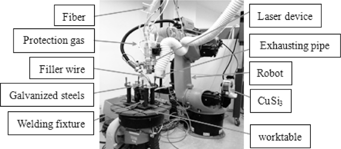
laser brazing system and experimental set-up.

National instrument company’s acquisition card NI USB-6212 and the signal conditioning board K-803B was used to measure the temperature of plate near the weld center. Figure 2 showed the sketch of the temperature measurement system.

Fig. 2.

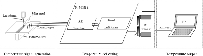
Schematic diagram of temperature measurement system.

3. The Establishment of Finite element Model

The volume mode was divided into the brazing seam zone, the transition zone and the zone far from the weld area. Figure 3 showed the sketch of the meshing of the volume model. The type of 3D solid70 thermal element was selected. The contradiction between computing accuracy and computing speed was been taken into account. The meshing is close in the brazing seam zone and transition area, on the contrary, thick away from the weld area.

Fig. 3.

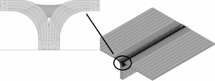
The sketch of the meshing of the volume model.

The following assumptions were required for modeling: (1) the room temperature is 20°C, (2) Without considering the wetting and spreading flow, and the material is continuous and isotropic, (3) The heat input of laser is not affected by the gas, (4) The energy distribution of the cross section of beam is Gauss distribution.

Laser brazing process is highly nonlinear transient, and the material thermal physical properties changes violently with the change of temperature. The differential equation of thermal conduction²²⁾ is   

$$\begin{array}{l}\frac{\partial }{\partial \left(\text{x}\right)}\left[\lambda \left(\text{T}\right)\frac{\partial \text{T}}{\partial \text{x}}\right]+\frac{\partial }{\partial \left(\text{y}\right)}\left[\lambda \left(\text{T}\right)\frac{\partial \text{T}}{\partial \text{y}}\right]+\frac{\partial }{\partial \left(\text{z}\right)}\left[\lambda \left(\text{T}\right)\frac{\partial \text{T}}{\partial \text{z}}\right]+\\ \text{Q}\left(\text{x,y,z,t}\right)=\rho c\left(\text{T}\right)\frac{\partial \text{T}}{\partial \text{t}}\end{array}$$(1)

In the formula (1), ρ, λ and c are respectively for material density, specific heat and thermal conductivity, they are functions of temperature; T is temperature; t is time; Q is internal heat source intensity. The birth-death element method was adopted to realize moving and loading of the laser energy. The seam elements were set to be death if the area of them were not be scanned by laser beam, the seam element was gradually activated with the moving of the laser beam. The elements located in the spot radius area were identified and picked up by APDL command stream. The simulation result of molten pool depth by the single Gauss heat source model is difficult to meet the requirements, and weld fusion lines does not match with laser brazing flange joint weld fusion lines. In addition, although the simulation result of molten pool width and depth can meet the requirements by double ellipsoid heat source model, weld fusion lines and laser brazing flange joint weld fusion lines does not match. So the composite heat source model of Gauss double ellipsoid was chosen to calculate, the improve heat source can simulate the energy distribution well, and the satisfactory shape of the weld pool can be obtained. The energy of the welding heat source was assigned to the two relatively independent heat source models in upper and lower interface, as is shown in formula (2). The sketch of heat source model is shown in Fig. 4.   

$$\{\begin{array}{l}\text{q(x,z)}=\frac{3\eta \text{P}}{\pi {\text{z}}_0{\hspace{0.17em}}^2}\times exp\left(-3\frac{{\text{x}}^2+{\text{z}}^2}{{\text{z}}_0{\hspace{0.17em}}^2}\right)\left(\text{y}\le 0\right)\\ \text{q}\left(\text{x,y,z}\right)=\frac{6\sqrt{3}{\mathrm{f}}_1\eta \text{P}}{{\text{abc}}_1\pi \sqrt{\pi }}\\ \hspace{0.5em}\hspace{1em}\hspace{1em}\hspace{1em}\times exp\left(\frac{-3{\text{x}}^2}{{\text{a}}^2}-\frac{3{\text{y}}^2}{{\text{b}}^2}-\frac{3{\left(\text{z}-{\text{z}}_0\right)}^2}{{\text{c}}_1{\hspace{0.17em}}^2}\right)\left(\text{y}>0,\text{z}\ge {\text{z}}_0\right)\\ \text{q}\left(\text{x,y,z}\right)=\frac{6\sqrt{3}{\mathrm{f}}_2\eta \text{P}}{{\text{abc}}_2\pi \sqrt{\pi }}\\ \hspace{0.5em}\hspace{1em}\hspace{1em}\hspace{1em}\times exp\left(\frac{-3{\text{x}}^2}{{\text{a}}^2}-\frac{3{\text{y}}^2}{{\text{b}}^2}-\frac{3{\left(\text{z}-{\text{z}}_0\right)}^2}{{\text{c}}_2{\hspace{0.17em}}^2}\right)\left(\text{y}>0,\text{z}<{\text{z}}_0\right)\end{array}$$(2)

Fig. 4.

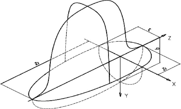
The sketch of heat source model of gauss double ellipsoid.

In the formula (2), η is laser absorptivity of material; f₁ and f₂ are total heat input in the front and rear half-ellipse, and f₁+f₂=2. In this study, the heat flux distribution parameters (a, b, c) were estimated according to the study of Tsai and Eagar.²³⁾ P is power; z₀ is z coordinate of heat source center.

When t=0 the initial temperature of workpiece is uniform and is equal to the environment temperature(T=T₀=20°C). In the process of laser brazing, laser area satisfy the second boundary condition.   

$$-\lambda \frac{\partial \text{T}}{\partial \text{n}}=\text{q}$$(3)

In the formula (3), n is normal direction of outside of the boundary surface.

At the symmetry surface, adiabatic boundary condition was considered:   

$$-\lambda \frac{\partial \text{T}}{\partial \text{n}}=0$$(4)

At the rest of the surface, convection heat transfer and radiation heat transfer was produced, so the third boundary condition was considered:   

$$-\lambda \frac{\partial \text{T}}{\partial \text{n}}=\beta \left(\text{T}-{\text{T}}_0\right)+\sigma \epsilon \left({\text{T}}^4-{\text{T}}_0{\hspace{0.17em}}^4\right)$$(5)

In the formula (5), T₀ is environment temperature; β is heat transfer coefficient; σ is Stefan-Boltzmann constant; ε is emissivity. Figure 5 showed variation of thermal-physical properties of base material with temperature.

Fig. 5.

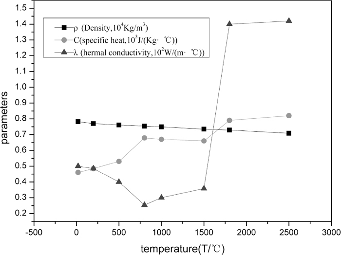
Thermal-physical properties of galvanized steel.

4. Response Surface Methodology

Response surface methodology (RSM) applies reasonable design of experimental to fit the functional relationships between the input factors and the response values, and concerns a set of mathematical and statistical techniques that are useful for modeling, analysis, predicting and optimization.²⁴⁾ RSM is used to establish the relationships between the welding process parameters and the responses based on the experimental data and then to predict responses and optimize the welding process parameters. In this paper, RSM was applied to the simulation data, and mathematical models was built using statistical software Design-expert V8.0.6.1. The effect of laser power, filler wire speed and brazing speed on the weld bead geometry was considered through RSM.

The simulation experiment was designed based on a three factors three levels Box-Behnken design with full replication.²⁵⁾ Laser power (1.2–2 kW), filler wire speed (1–1.4 m/min) and brazing speed (0.72–1.2 m/min) represent the laser independent input variables. Table 4 shows laser input variables and experimental design levels used.

Table 4. Independent variable and experimental design levels used.

Variable	Unit	Code
		Low (−1)	Medium (0)	High (+1)
Laser power (P)	KW	1.2	1.6	2
filler wire speed (V1)	m/min	1	1.2	1.4
brazing speed (V2)	m/min	0.72	0.96	1.2

5. Results and Discussion

5.1. Temperature Field Simulation and Experimental Measurement

Figures 6(a)–6(c) shows the calculated temperature field at different time at the laser power of 1600 W, brazing speed of 0.96 m/min, defocusing distance of 30 mm. Temperature contour map of longitudinal section (Fig. 7) was given to obtain weld bead geometry at different process conditions. Weld bead geometry is obtained according to the melting point (1025°C) of solder as optimizing samples.

Fig. 6.

Brazing temperature distribution map of different time.

Fig. 7.

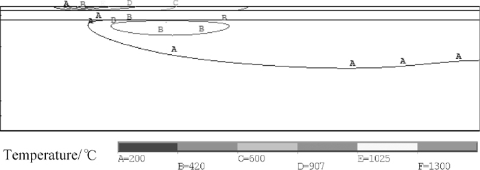
Temperature contour map of longitudinal section.

Figure 8 shows that experimental result (a)–(c) had similar cross sectional geometry with simulation joint (d)–(e) in different laser power, indicating that the geometric model establishment method was reasonable in most conditions. The temperature field on the interface between two plates was also symmetric.

Fig. 8.

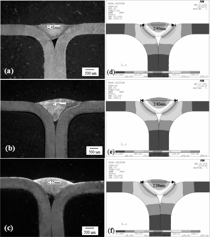
Cross section of simulation and experiment: (a), (d) P=1600 W; (b), (e) P=2000 W; (c), (f) P=1200 W.

The filling content of solder and temperature field distribution were influenced by different laser power. When P=1600 W, the surface morphology was smooth, and the quality of seam forming was well, as is shown in Fig. 8(a). The temperature field nephogram shows the peak temperature was lower, and temperature field distribution was also uniform. When P=2000 W, laser power was too high, the solder was overheated due to high power density. The temperature field nephogram shows temperature gradient and the area of high temperature were too large, as is shown in Fig. 8(e). When P=1200 W, laser power was low, the liquidity of solder was poor, so the quality of seam forming was not so well, as is shown in Fig. 8(c). The temperature field nephogram shows the peak temperature was not high enough to melt solder.

The SEM images of the joint interface between base metal and filler metal in the middle of braze seam were showed in Fig. 9. And the EDS analysis is carried out to obtain the components of positions D, E and F, the results are listed in Table 5. We can find that the dispersive phases at the position D, E, F enriches in Si, Fe and Cu. The particle phases can be identified as intermetallic compounds of Si, Fe and Cu. Besides, the content of intermetallic compounds increased with the increase of the laser power. This is because the elements are apt to concentrate at the interface layer in high heat input mode. With a thin interface layer (<10 μm), large brittle phases can be avoided and the performance of welding joint was improved. In the study, no large brittle phases were found and a good brazing joint was obtained.

Fig. 9.

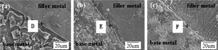
SEM of braze seam with different laser power: (a) 1200 W (b) 1600 W (c) 2000 W.

Table 5. Compositions of positions in Fig. 9 (mass fraction, %).

Position	Si	Fe	Cu
D	9.40	15.19	75.41
E	8.24	3.20	88.56
F	5.33	4.36	90.31

To evaluate the accuracy of the simulation results of temperature field, the experiment of temperature measurement was carried out to compare. Due to the temperature of the weld area is difficult to measure, the experiment took three points near the weld center, as is shown in Fig. 10. Thermocouple was adopted to measure the temperature change of brazing process. Thermal cycle curve was drawn, and the test results was compared with simulation results. As is described in Fig. 11, comparison showed that the experimental results had good agreement with calculated results. Heating rate and peak temperature of A, B and C points are consistent with simulation results. But the agreement between experiment and simulation results was not satisfied in the cooling process. The main reason is that laser heating process was simplified in calculation process. The effect of solder internal flowing on heat transfer and the effect of shielding gas on weld cooling were not considered.

Fig. 10.

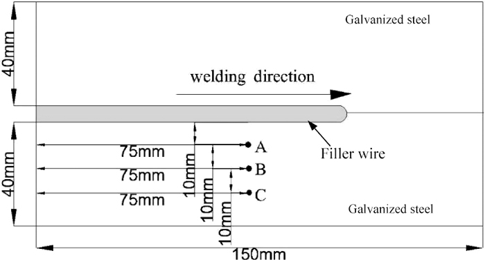
Schematic diagram of position of dot in plate.

Fig. 11.

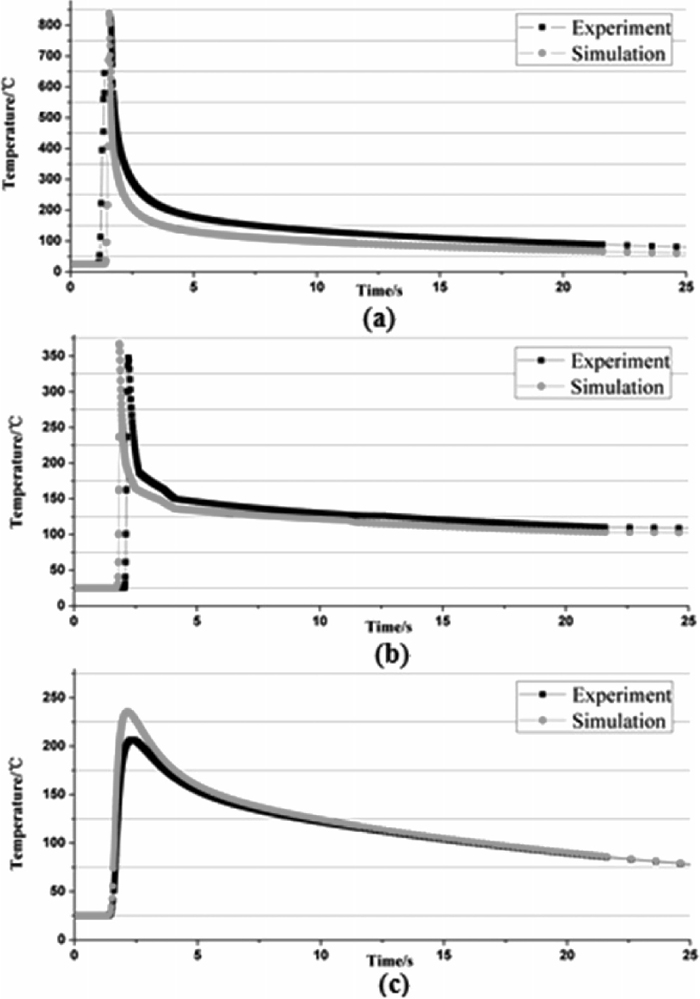
Comparison of measured temperature values and simulation temperature values: (a) Temperature cycling curve of point A; (b) Temperature cycling curve of point B; (c) Temperature cycling curve of point C.

5.2. Parameters Optimization

According to the content mentioned in section 5.1, weld bead geometry of different brazing conditions were measured through the temperature contour map of longitudinal section. From all samples, 17 groups were selected as optimizing samples to built mathematical models based on Box-Behnken Design, as is shown in Table 6. The weld bead geometry parameters of flange joint include weld width(WW), weld penetration(WP), as shown in Fig. 12.

Table 6. Orthogonal simulation experiment.

Std	Value			Weld profile geometry
	P (KW)	V1 (m/min)	V2 (m/min)	WW (mm)	WP (mm)
1	1.60	1.40	1.20	1.654	0.862
2	1.60	1.20	0.96	1.825	0.752
3	2.00	1.20	0.72	2.325	0.932
4	1.20	1.00	0.96	1.524	0.769
5	2.00	1.00	0.96	2.114	0.946
6	2.00	1.40	0.96	2.425	0.965
7	1.60	1.20	0.96	1.875	0.816
8	1.60	1.40	0.72	1.641	0.879
9	1.60	1.00	1.20	1.722	0.813
10	1.60	1.20	0.96	1.935	0.841
11	1.20	1.20	1.20	1.698	0.789
12	1.60	1.20	0.96	1.863	0.851
13	1.20	1.20	0.72	1.567	0.762
14	2.00	1.20	1.20	2.364	0.997
15	1.60	1.00	0.72	1.798	0.821
16	1.20	1.40	0.96	1.679	0.831
17	1.60	1.20	0.96	1.905	0.792

Fig. 12.

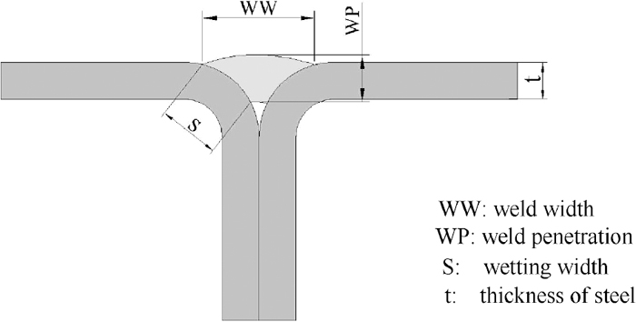
Schematic diagram of weld bead geometry of flang butt joints.

5.2.1. Effect of Process Factor on Weld Width

Design-Expert V8.0.6.1 software is used for analysis of the measured responses and testing the adequacy of the mathematical models using the analysis-of-variance (ANOVA) technique.²⁶⁾ The sequential f-test, lack-of-fit test and R²-test were carried out. The F-test for significance on individual model coefficients, if values of “Prob > F” greater than 0.1000, which indicate model terms are not significant and values less than 0.0500 indicate the model terms are significant. The R²-test implies the goodness of fits for the model that the more closely R² is to 1, more accurate the model is. And the “Pred R-Squared” is in reasonable agreement with the “Adj R-Squared” and are close to 1, which indicate adequacy of the model.²⁷⁾ “Adeq Precision” indicates the signal to noise ratio. A ratio greater than 4 is desirable. The analysis of variance of each response is shown in Table 7.

Table 7. ANOVA for weld width reduced Quadratic Model.

Source	Sum of squares	df	Mean square	F value	Prob > F
Model	1.15	9	0.13	12.07	0.0017	Sign.
A-P	0.95	1	0.95	89.56	<0.0001
B-V1	7.260E-003	1	7.260E-003	0.68	0.4359
C-V2	1.431E-003	1	1.431E-003	0.13	0.7245
AB	6.084E-003	1	6.084E-003	0.57	0.4741
AC	2.116E-003	1	2.116E-003	0.20	0.6690
BC	1.980E-003	1	1.980E-003	0.19	0.6790
A2	0.12	1	0.12	11.42	0.0118
B2	0.056	1	0.056	5.23	0.0561
C2	0.016	1	0.016	1.52	0.2576
Residual	0.074	7	0.011
Lack of Fit	0.067	3	0.022	12.87	0.0160	Sign.
Pure Error	6.987E-003	4	1.747E-003
Cor Total	1.23	16

R2=0.9394, Adj R2=0.8616, Pred R2=0.8132, Adeq Precision=9.711

Table 7 for the reduced quadratic model summarizes the analysis of variance of WW which eliminates the insignificant model terms automatically by selecting the step-wise regression method. The Model F-value of 12.07 implies the model is significant. There is only a 0.17% chance that a “Model F-Value” this large could occur due to noise. In this case P, P² are significant model terms. The “Lack of Fit F-value” of 12.87 implies the Lack of Fit is significant. There is only a 1.6% chance that a “Lack of Fit F-value” this large could occur due to noise. The determination coefficient R²=0.9394 was also shown in Table 7, and the “Pred R-Squared” of 0.8616 is in reasonable agreement with the “Adj R-Squared” of 0.8132. And “Adeq Precision” ratio of 9.711 above 4 indicates adequate model discrimination. The analysis of variance indicates that this model can be used to navigate the design space.

The final mathematical models for weld width, WW, in terms of coded factors as determined by design expert software are:   

$$\begin{array}{l}\text{WW}=1.88+0.35\text{P}+0.030{\text{V}}_1+0.013{\text{V}}_2+0.039{\text{PV}}_1\\ -\hspace{0.17em}\hspace{0.17em}0.023{\text{PV}}_2+0.022{\text{V}}_1{\text{V}}_2+0.17{\text{P}}^2-0.11{\text{V}}_1{\hspace{0.17em}}^2-0.062{\text{V}}_2{\hspace{0.17em}}^2\end{array}$$(6)

While the following final empirical models in terms of actual factors are:   

$$\begin{array}{l}\text{WW}=8.98-14.27\text{P}+4.85{\text{V}}_1+2.43{\text{V}}_2+0.98{\text{PV}}_1\\ -\hspace{0.17em}\hspace{0.17em}0.48{\text{PV}}_2+0.46{\text{V}}_1{\text{V}}_2+4.25{\text{P}}^2-2.87{\text{V}}_1{\hspace{0.17em}}^2-1.08{\text{V}}_2{\hspace{0.17em}}^2\end{array}$$(7)

The perturbation plot for the WW is shown in Fig. 13. It is clear that the WW increases with increase in laser power, similarly, WW decreases with increase in filler wire speed in the second half. The laser power is the most significant factor affecting the WW. Figure 14 shows the response surface (3D) and the contour graph (2D) effect of the laser power and filler wire speed on the WW at the brazing speed equal to 0.96 m/min. From Fig. 14(a) it can be seen WW decreases with increase in filler wire speed when filler wire speed is more than 1.20 m/min. Figure 15 presents the interactions between brazing speed and filler wire speed on WW, when laser power at 1.6 KW. It can be ascertained filler wire speed at lower or higher level contribute to decreasing WW, and if keeping laser powder and filler wire speed at higher level, the higher WW can be obtained.

Fig. 13.

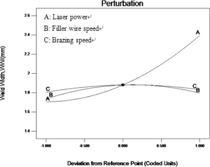
Perturbation plot showing the effect of all factors on weld width.

Fig. 14.

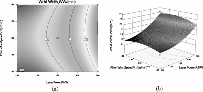
The effect of laser power and filler wire speed on weld width.

Fig. 15.

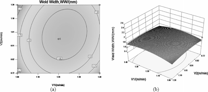
The effect of filler wire speed and brazing speed on weld width.

5.2.2. Effect of Process Factor on Weld Penetration

For weld penetration, the fit summary recommends the cubic model where the additional terms are significant and the model is aliased. The ANOVA table of the cubic model which eliminates the insignificant model terms automatically was presented by selecting the step-wise regression method in Table 8. As shown in Table 7, the Model F-value of 12.56 implies the model is significant. In this case P are significant model terms. The determination coefficient R²= 0.7436 close to 1.00 and the predicted R² is in reasonable agreement with the adjusted R². The ratio of “Adeq Precision” is greater than 4. All of analysis indicates an adequate signal. This model can be used to navigate the design space.

Table 8. ANOVA for weld penetration reduced Linear Model.

Source	Sum of Squares	df	Mean Square	F Value	Prob > F
Model	0.064	3	0.021	12.56	0.0004	Sign.
A-P	0.059	1	0.059	34.78	<0.0001
B-V1	4.418E-003	1	4.418E-003	2.59	0.1316
C-V2	5.611E-004	1	5.611E-004	0.33	0.5761
Residual	0.022	13	1.706E-003
Lack of Fit	0.016	9	1.757E-003	1.10	0.4998
Pure Error	6.365E-003	4	1.591E-003
Cor Total	0.087	16

R²= 0.7436, Adj R²= 0.6844, Pred R²= 0.6135, Adeq Precision=10.942

The final mathematical models for weld penetration, WP, in terms of coded factors as determined by design expert software are:   

$$\text{WP}=0.85+0.086\text{P}+0.024{\text{V}}_1+8.375\text{E}-003{\text{V}}_2$$(8)

While the following final empirical models in terms of actual factors are:   

$$\text{WP}=-0.102+0.431\text{P}+0.118{\text{V}}_1+0.035{\text{V}}_2$$(9)

Figure 16 is a perturbation plot, which illustrates the effect of all the factors on WP. The WP of laser brazing is closely related to laser power and filler wire speed. It is evident that laser power, filler wire speed and brazing speed have a positive effect on the WP. In fact, increasing of laser power and filler wire speed make the WP of laser brazing to increase. The laser power is the most significant factor affecting WP, and then is filler wire speed, while the brazing speed affects WP just slightly. Figure 17 illustrates the Interaction effects of laser power and filler wire speed on WP. The parameter brazing speed on 0.96 m/min. From the response surface, as shown Fig. 17(b), the influence of process parameters on the WP can be more directly perceived to see, which indicates that the results is consistent with perturbation plot. While from the contour graph, as shown Fig. 17(a), different combinations of parameters can achieve the same response value, which means the process parameters can be optimized according to the divided region by the contour lines.

Fig. 16.

Perturbation plot showing the effect of all factors on weld penetration.

Fig. 17.

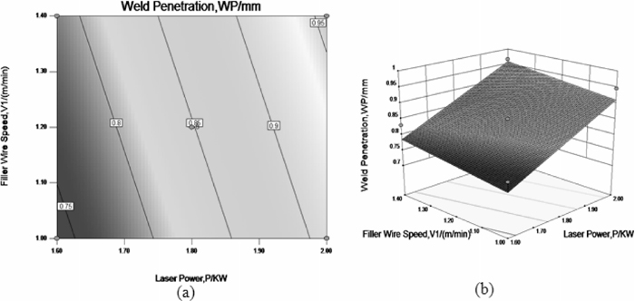
The effect of laser power and filler wire speed on weld penetration.

5.2.3. Validation of the Models

The relationship between the actual and predicted values of WW and WP was exhibited in Fig. 18. It is obvious that the predicted values of the developed models are in good agreement with the actual values. The models are adequate as a result of that the residuals tend to be close to the diagonal line.

Fig. 18.

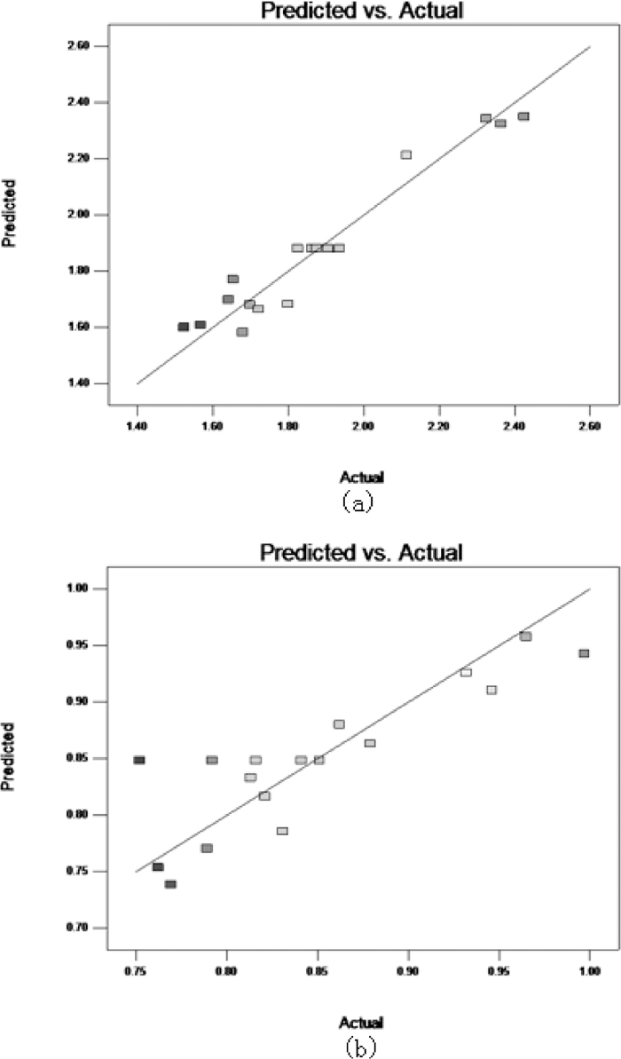
Relationship between experimental and predicted values: (a) weld width; (b) weld penetration.

In addition, three confirmation experiments were carried out with welding conditions chosen randomly within the experiment range to validate the developed models. Table 9 exhibits the experiments condition, actual results, predicted values and calculated percentage error of confirmation experiments. The predicted values of WW and WP were calculated using the previous developed models. From the confirmation experiments results, it indicates that the maximum predicted errors of WW and WP are 2.72% and 2.41%, respectively. All the error values are in the range of engineering errors and accepted in the industry.

Table 9. Confirmation experiments of the WW and WP responses.

Exp. No.	P, KW	V1, m/min	V2, m/min	WW, mm		|E|, %	WP, mm		|E|, %
				Act.	Pred.		Act.	Pred.
1	1.97	1.39	1.2	2.265	2.205	2.72	0.968	0.952	1.68
2	1.97	1.37	1.2	2.259	2.228	1.39	0.942	0.950	0.84
3	1.98	1.39	1.18	2.213	2.240	1.21	0.978	0.955	2.41

5.2.4. Optimization

Desirability function approach is simple, available in software and flexibility to deal with the optimization of multi-objective responses through transforming a multiple response problem into a single response problem.

The optimization process involves combining the goals into the overall desirability function. Meanwhile, the numerical optimization would find one point or more that maximize this function. In the numerical optimization criteria was implemented. For every response there is a different importance, according to the required goal. According to the method, Design Expert statistical software package is utilized again for the optimization operation. Table 10 shows the optimal laser brazing conditions according to the criterion, which will lead to maximum predicted WW of about 2.241 mm and WP of about 0.958 mm.

Table 10. Optimal solution.

Number	P	V1	V2	WW		WP		Desirability
				Cal.	Exp.	Cal.	Exp.
1	1.6	1.19	0.96	2.220	2.219	0.955	0.954	1.00
2	1.6	1.19	0.95	2.236	2.233	0.955	0.953	1.00
3	1.6	1.20	0.95	2.241	2.243	0.958	0.955	1.00

6. Conclusion

(1) The heat source model can reflect the features of actual laser brazing process. The calculated results were in good agreement with the experimental results.

(2) Through numerical calculation, the temperature of different position near the weld center on the workpiece surface was consistent with the temperature of synchronous measurement.

(3) The developed mathematical models of the weld bead geometry can be used to predict the responses adequately within the limits of welding parameters being used.

(4) The optimal welding condition can be determined effectively using the numerical optimization technique, which results in a set of optimal solutions according to the desired optimization criteria.

Acknowledgements

This research was supported by Foundation of Natural Science Foundation of China (51375294), Local College Capacity Building of Shanghai Science and Technology Committee (13160501200), Research Innovation Project of Shanghai Education Committee (14YZ139), Foundation of Shanghai University of Engineering Science (2012gp21), Graduate student research innovation of Shanghai University of Engineering Science(14KY0507, 14KY0509).

References

• 1)   M.  Heitmanek,  M.  Dobler,  M.  Graudenza,  W.  Perret,  G.  Göbel,  M.  Schmidt and  E.  Beyer: Phys. Procedia, 56 (2014), 689.
• 2)   L.  Rodriguez,  A.  Mathieu,  C.  Langlade,  A.  Vannes,  D.  Grevey and  S.  Mattei: Lasers. Eng., 15 (2005), 413.
• 3)   A.  Grimm: Fertigungstechnik Erlangen * Band, 229 (2012), Seite 1.
• 4)   D.  Deng and  H.  Murakawa: J. Comput. Mater. Sci., 37 (2006), 209.
• 5)   S. A.  Tsirkas,  P.  Papanikos and  T.  Kermanidis: J. Mater. Process. Technol., 134 (2003), 59.
• 6)   G.  Verhaeghe: Predictive Formulate for Weld Distortion-A Critical Review, Woodhead Publishing, England, (1999), 1.
• 7)   C. H.  Lee and  K. H.  Chang: J. Appl. Therm. Eng., 45 (2012), 33.
• 8)   T. L.  Teng,  C. P.  Fung,  P. H.  Chang and  W. C.  Yang: Int. J. Press. Vessel. Pip., 78 (2001), 523.
• 9)   D.  Deng,  W.  Liang and  H.  Murakawa: J. Mater. Process. Technol., 183 (2007), 219.
• 10)   Z.  Barsoum and  A.  Lundback: Eng. Fail. Anal., 16 (2009), 2281.
• 11)   J.  Goldak,  A.  Chakravarti and  M.  Bibby: Metall. Trans. B, 15B (1984), 299.
• 12)   J.  Mazumder and  W. M.  Steen: J. Appl. Phys., 51 (1980), 941.
• 13)   D. T.  Swift-Hook and  A. E. F.  Gick: Weld. J., 52 (1973), 492.
• 14)   J.  Dowden,  M.  Davis and  P.  Kapadia: J. Fluid. Mech., 126 (1983), 123.
• 15)   K. N.  Lankalapalli,  J. F.  Tu and  M.  Gartner: J. Appl. Phys., 29 (1996), 1831.
• 16)   J.  Park and  S.  Na: Weld. J., 77 (1998), 155.
• 17)   P.  Peyre,  G.  Sierra,  F.  Deschaux-Beaume,  D.  Stuart and  G.  Fras: Mater. Sci. Eng. A, 444 (2007), 327.
• 18)   A.  Mathieu,  S.  Matteï,  A.  Deschamps,  B.  Martin and  D.  Grevey: NDT & E Int., 39 (2006), 272.
• 19)   K. Y.  Benyounis,  A. G.  Olabi and  M. S. J.  Hashmi: Opt. Laser Technol., 40 (2008), 76.
• 20)   A. G.  Olabi,  G.  Casalion,  K. Y.  Benyounis and  M. S. J.  Hashmi: Mater. Des., 28 (2007), 2295.
• 21)   H. A.  Eltawahni,  A. G.  Olabi and  K. Y.  Benyounis: Opt. Laser Technol., 43 (2011), 648.
• 22)   Q.-c.  Chu,  X.-l.  He and  G.  Yu: Chin. J. Laser, 37 (2010), 3180.
• 23)   N.  Tsai and  T.  Eagar: Metall. Trans. B, 16 (1985), 841.
• 24)   D. C.  Montgomery: Design and Analysis of Experiments. 5th ed., Wiley, New York, (2001), 1.
• 25)  Stat-Ease Inc.: Design-Expert Software, v7, User’s Guide, Technical Manual, Stat-Ease Inc., Minneapolis, MN, (2000), 1.
• 26)   A.  Ghosal and  A.  Manna: Opt. Laser Technol., 46 (2013), 67.
• 27)   B.  Acherjee,  D.  Misra,  D.  Bose and  K.  Venkadeshwaran: Opt. Laser Technol., 41 (2009), 956.