Scaling Physical Model Study on Dynamic Accumulation of Bottom Dross in a Molten Zinc Pot

Abstract

A theoretical framework of similarity and its related experimental methods concerning scaling physical model are presented to investigate dynamic behavior of bottom dross in a zinc pot during the continuous hot-dip galvanizing process. Based on the similarity criteria of Froude number, turbulent Reynolds number, Shields number and particle Reynolds number, an analytical framework is developed to describe similarity of dross dispersion, transport and deposition in a stirred molten zinc tank. A complete set of experimental methods are suggested correspondingly. A 1/5 reduced scale model is adopted to study steady flow field, dynamic accumulation rules and stable shape of bottom dross. NaCl aqueous solutions and black particles of acrylonitrile butadiene styrene are employed as model fluid and bottom dross, respectively. The results show that two impact flows are the key factors in the formation of dross deposition morphology in the bottom of zinc bath. The first impact flow strikes bottom drosses located in the floor of tank and near the front wall and results in three impact craters for symmetric distribution. The other impact flow hits bottom drosses deposited blow the sink roll. A pair of pits with curved edges and a ridge between them are formed. The dispersed bottom drosses under impact are carried by the main circular flow and heaped up toward the back wall similar to a mobile dune. The greater the difference between current shape and steady state morphology of bottom dross, the more dross particles are scattered.

1. Introduction

In a continuous hot-dip galvanizing line the strip submerged in the Zn pot moves around a sink roll and a pair of support rolls.¹⁾ Dross is generated due to metallic compounds and chemical reactions occurring in the zinc bath²⁾ and sorted into top dross, free dross and bottom dross according to the density ratio of dross to liquid zinc. Dross, especially the bottom dross, pick-up on steel strip is a common coating defect in hot dip galvanizing and therefore lowers the surface quality of steel sheets.³⁾ For purpose of development of bottom dross control technologies, research on the dynamic accumulation behaviors of bottom dross in the zinc pot, including dispersion, transport and deposition, should be carried out. This is the main content of this paper.

Physical model experiments are usually employed to observe as well as measure complex systems directly. Several experimental devices were designed and used to determine the circulation patterns of molten metal in the zinc pot.^4,5) In the lab, a reduced scale model made of transparent material was generally used to facilitate measurements. The flow pattern, mean flow velocity components, root-mean-square values of turbulence components and Reynolds shear stress were obtained.⁶⁾ Nonetheless, special requirements of PIV (Particle Image Velocimetry) and LDV (Laser Doppler Velocimetry) for visualization particles make them only fit investigations on the flow field without dross. Dynamic accumulation behaviors of bottom dross involve problems on solid-liquid two-phase turbulent flow. In metallurgical industry, the most typical research associated with it was focus on floatation, agglomeration and removal of nonmetallic inclusions in the tundish.^7,8) Similarity between prototype and water model was mainly based on two criterion frameworks. One developed a relationship to provide the similarity of inclusion trajectories between water model and prototype. The equations were derived in the light of the synthetic motion theorem of points and Froude similarity criterion.^7,9,10) The other maintained similar movement of inclusions on the basis of modified Froude number^11,12) or plume Froude number.^13,14) Few studies on physical model experiments for dynamic behaviors of bottom dross were conducted in literatures. The unique public report on interrelated research gotten by authors was performed by Jun Kurobe.^15,16) The investigation using a reduced scale cold model was focused on streak lines of top and bottom dross in the flow field of a plating bath. Modified Froude number was selected as the unique similarity criterion to provide a dynamic similitude for determining the size and density of the model dross.¹⁷⁾ A small amount of solid particles were supplied from liquid surface to observe the motions of dross by eye inspection. Experimental methods in the literature,¹⁶⁾ especially for the choice of model fluid, inspired research of this manuscript despite deviations between experimental results and prototype due to the crude similitude and influence of immersed sensors on the flow field in the bath. Until now, studies on dynamic accumulations and distributions of bottom drosses in the floor of zinc pot have not been reported.

The main purpose of this manuscript is to develop a similarity framework and a series of corresponding experimental approaches for scaling physical model experiments aiming at the investigation on dynamic accumulations and distributions of bottom drosses in a continuous hot-dip galvanizing bath. With different quantities of bottom dross, evolution rules of dynamic deposition and steady morphologies are probed. The basis of field productions concerning optimization for monitoring scheme and control technologies of bottom dross is provided.

2. Similarity Framework

2.1. Similarity Criteria for Molten Zinc Flow

It is well known that the flow field and particle movements of model cannot be identical to that of prototype due to failing to meet all the similarity laws simultaneously. Geometric and dynamic similarities between the scale model and its real-world prototype are mainly taken into account in this manuscript. In general, geometric similarity (see Eq. (1)) is confirmed on account of pre-existing test conditions.   

$$\lambda =\frac{L_{\text{m}}}{L_{\text{p}}}$$(1)

where λ represents the geometric similarity ratio between the model and its prototype, L denotes a characteristic length and the diameter of sink roll is selected as the characteristic length due to being a stirred vessel system. Subscripts m and p signify model and prototype respectively.

As a representation of viscous flow characteristics, the Reynolds number (Re, see Eq. (2)) is the ratio of the inertial forces to the viscous forces.   

$${\text{R}}_{\text{e}}=\frac{VL}{\upsilon }$$(2)

where V and υ are flow velocity and kinematic viscosity of the fluid respectively. The Reynolds number plays a vital role in experiments of fluid mechanics involving the influence of viscidity. The Froude number (Fr, see Eq. (3)), characterizing the flow due to gravity, is defined as   

$$\text{Fr}=\frac{V^2}{\text{g}L}$$(3)

where g denotes gravity constant. Considering Eqs. (1) and (3), similitude between model and prototype according to the Froude number is given by expression Eq. (4).   

$$V_{\text{m}}=\sqrt{\lambda }\hspace{0.17em}{V}_{\text{p}}$$(4)

Based on Froude similarity criterion, the time scale governing the flow can be written as   

$$\frac{T_{\text{m}}}{T_{\text{p}}}=\frac{L_{\text{m}}{V}_{\text{p}}}{L_{\text{p}}{V}_{\text{m}}}=\sqrt{\lambda }$$(5)

where, T_m and T_p are called time of model and prototype, respectively. In general, meeting Reynolds and Froude similarity criteria simultaneously is not usually feasible in model experiments at room temperature. If the flow regimes of the model and prototype are all in the second automatic simulation region (namely the turbulent-flow region), flow regimes and velocity distributions are not governed by the Reynolds number any more. The flow Reynolds number can be relaxed under fully turbulent conditions in both prototype and model. That is to say, the turbulent Reynolds number similarity criterion is naturally satisfied if one operates in the turbulent regime.⁷⁾ So, to remain dynamic similitude, only the Froude numbers of the model and the prototype are required to keep equal.

2.2. Similarity Criteria for Bottom Dross Movement

On the basis of flow field similitude between model and prototype carrier fluids, parameters of the model carrier fluid and appropriate particles are further confirmed to simulate dynamic behaviors of bottom dross such as dispersion, transport and accumulation. In this study, a scaling approach based on similarities of the Shields and particle Reynolds numbers is presented. In the flow field of zinc pot, steady-state movements for the dispersed bottom drosses under impacts may be regarded as the particles flow of dilute concentrations. So a simplification is introduced since the liquid zinc and particle dynamic are decoupled. The flow of liquid zinc may be considered regardless of the inclusion flow. The motion of a rigid particle in a viscous flow may be described by the BBO (Basset–Boussinesq–Oseen) equation.^18,19) This ordinary differential equation can be reduced to Eq. (6) without regard to Basset force.   

$$\begin{array}{l}{\rho }_{\text{inc}}\frac{\text{d}{\mathit{V}}_{\text{inc}}}{\text{d}t}={\rho }_{\text{f}}\frac{\text{d}{\mathit{V}}_{\text{f}}}{\text{d}t}+\left({\rho }_{\text{inc}}-{\rho }_{\text{f}}\right)\mathbf{g}\\ +\frac{3{\rho }_{\text{f}}}{4D_{\text{inc}}}{C}_{\text{d}}\left|{\mathit{V}}_{\text{f}}-{\mathit{V}}_{\text{inc}}\right|\left({\mathit{V}}_{\text{f}}-{\mathit{V}}_{\text{inc}}\right)-\frac{{\rho }_{\text{f}}}{2}\frac{\text{d}\left({\mathit{V}}_{\text{inc}}-{\mathit{V}}_{\text{f}}\right)}{\text{d}t}\end{array}$$(6)

where ρ_inc and ρ_f represent densities of inclusion and fluid respectively, subscripts f and inc denote fluid and increment, V_inc and V_f are absolute-velocity vectors of particle and fluid, g is the acceleration due to gravity, D_inc signifies diameter of inclusion/bottom dross, the particles are assumed to be rigid and have a spherical shape, C_d is called drag coefficient. Terms on the right hand side, in turn, represent the inertial force, the buoyancy force, the drag force and the added mass force. If the value of ρ_inc is close to ρ_f, Eq. (6) can be simplified and rearranged as   

$$\frac{3}{2}{\rho }_{\text{f}}\frac{\text{d}\left({\mathit{V}}_{\text{inc}}-{\mathit{V}}_{\text{f}}\right)}{\text{d}t}=\left({\rho }_{\text{inc}}-{\rho }_{\text{f}}\right)\mathbf{g}+\frac{3{\rho }_{\text{f}}}{4D_{\text{inc}}}{C}_{\text{d}}\left|{\mathit{V}}_{\text{f}}-{\mathit{V}}_{\text{inc}}\right|\left({\mathit{V}}_{\text{f}}-{\mathit{V}}_{\text{inc}}\right)$$(7)

The drag coefficient C_d is found to depend on the particle Reynolds number Re_inc (shown in Eq. (8)). It also can be obtained experimentally and approximated by.²⁰⁾   

$${\text{Re}}_{\text{inc}}=\frac{\left|{\mathit{V}}_{\text{inc}}-{\mathit{V}}_{\text{f}}\right|D_{\text{inc}}}{{\upsilon }_{\text{f}}}$$(8)

where υ_f is the kinematic viscosity of a fluid. For a small particle Reynolds number, the drag coefficient (see Eq. (9)) is inversely proportional to Re_inc according to Stokes’ proposal in 1851.   

$$C_{\text{d}}=\frac{24}{{\text{Re}}_{\text{inc}}}$$(9)

Substituting Eqs. (8) and (9) to Eq. (7) yields   

$$\frac{\text{d}\left({\mathit{V}}_{\text{inc}}-{\mathit{V}}_{\text{f}}\right)}{\text{d}t}+\frac{12{\upsilon }_{\text{f}}}{D_{\text{inc}}^2}\left({\mathit{V}}_{\text{inc}}-{\mathit{V}}_{\text{f}}\right)=\frac{2}{3}\left(\frac{{\rho }_{\text{inc}}}{{\rho }_{\text{f}}}-1\right)\mathbf{g}$$(10)

According to Eq. (10), the analytical solution for the relative speed with zero initial conditions is given by   

$$\left({\mathit{V}}_{\text{inc}}-{\mathit{V}}_{\text{f}}\right)=\frac{D_{\text{inc}}^2}{18{\upsilon }_{\text{f}}}\left(\frac{{\rho }_{\text{inc}}}{{\rho }_{\text{f}}}-1\right)\left(1-{\text{e}}^{\frac{-12{\upsilon }_{\text{f}}}{D_{\text{inc}}^2}t}\right)\mathbf{g}$$(11)

Equation (11) shows, under zero initial conditions, the direction of relative velocity between inclusions and the fluid is the same as the acceleration due to gravity. This is similar to a falling sphere in a static fluid. Plugging Eq. (11) into Eq. (8) and considering steady state for time approaching infinity as well, particle Reynolds number is rewritten as   

$${\text{Re}}_{\text{inc}}=\frac{D_{\text{inc}}^3}{18{\upsilon }_{\text{f}}^2}\left(\frac{{\rho }_{\text{inc}}}{{\rho }_{\text{f}}}-1\right)\text{g}$$(12)

The particle Reynolds number is important as considering the fall velocity of sediment. In order to achieve the similarity between model and prototype, the particle Reynolds number should be preserved identically (see Eq. (13)) when its value is not high enough to ensure the flow is fully hydrodynamically rough.   

$$\frac{D_{\text{inc,}\mathrm{\hspace{0.17em} }\text{m}}^3{\upsilon }_{\text{f,}\mathrm{\hspace{0.17em} }\text{p}}^2}{D_{\text{inc,}\mathrm{\hspace{0.17em} }\text{p}}^3{\upsilon }_{\text{f,}\mathrm{\hspace{0.17em} }\text{m}}^2}=\frac{\left(\frac{{\rho }_{\text{inc,}\mathrm{\hspace{0.17em} }\text{p}}}{{\rho }_{\text{f,}\mathrm{\hspace{0.17em} }\text{p}}}-1\right)}{\left(\frac{{\rho }_{\text{inc,}\mathrm{\hspace{0.17em} }\text{m}}}{{\rho }_{\text{f,}\mathrm{\hspace{0.17em} }\text{m}}}-1\right)}$$(13)

Shields number θ is another key parameter used for guaranteeing similarity of scaling sediment motion between prototype and model. The Shields number, also called the Shields criterion, is a nondimensional number to calculate the initiation of motion of sediment in a fluid flow. It is regarded as the ratio of fluid force on the particle to the weight of the particle and given in the following form²¹⁾   

$$\theta =\frac{{\rho }_{\text{f}}{V}^2}{D_{\text{inc}}\left({\rho }_{\text{inc}}-{\rho }_{\text{f}}\right)\text{g}}$$(14)

Based on the same Shields number, the similarity criterion of sediment movement between prototype and model can be expressed as (see Eq. (15))   

$$\frac{D_{\text{inc,}\mathrm{\hspace{0.17em} }\text{m}}{V}_{\text{p}}^2}{D_{\text{inc,}\mathrm{\hspace{0.17em} }\text{p}}{V}_{\text{m}}^2}=\frac{\left(\frac{{\rho }_{\text{inc,}\mathrm{\hspace{0.17em} }\text{p}}}{{\rho }_{\text{f,}\mathrm{\hspace{0.17em} }\text{p}}}-1\right)}{\left(\frac{{\rho }_{\text{inc,}\mathrm{\hspace{0.17em} }\text{m}}}{{\rho }_{\text{f,}\mathrm{\hspace{0.17em} }\text{m}}}-1\right)}$$(15)

Given the above, in addition to geometric similarity (see Eq. (1)), the framework of scaling criteria for the physical model investigation on dynamic behavior of bottom dross in the zinc pot contains similarities of Froude number (see Eq. (4)), particle Reynolds number (see Eq. (13)) and Shields number (see Eq. (15)). Similarity criterion of Reynolds number is relaxed when Re is high enough to establish fully turbulent conditions. That may also be called “turbulent Reynolds number similarity criterion”. The three similarity criteria (see Eqs. (4), (13) and (15)) are employed to determine parameters of scaling physical model. Dividing Eq. (13) by the cube of Eq. (15) and introducing Eqs. (4), (16) is deduced   

$${\upsilon }_{\text{f, m}}\left(\frac{{\rho }_{\text{inc,}\mathrm{\hspace{0.17em} }\text{m}}}{{\rho }_{\text{f,}\mathrm{\hspace{0.17em} }\text{m}}}-1\right)={\upsilon }_{\text{f,}\mathrm{\hspace{0.17em} }\text{p}}\left(\frac{{\rho }_{\text{inc,}\mathrm{\hspace{0.17em} }\text{p}}}{{\rho }_{\text{f,}\mathrm{\hspace{0.17em} }\text{p}}}-1\right){\lambda }^{\frac{3}{2}}$$(16)

During the process of determinations on the physical model, the precondition of Eq. (7), namely guaranteeing ρ_{inc, m} close to ρ_{f, m}, and the relevance between ρ_{f, m} and υ_{f, m} should be taken into account synchronously. Given the geometric similarity ratio λ, materials of the model fluid and bottom dross, that is ρ_{f, m}, ρ_{inc, m} and υ_{f, m}, may be ascertained firstly according to Eq. (16). So D_{inc, m} is deduced from Eq. (13) and then V_m is calculated by Eq. (4). In the end, the model fluid is verified whether it is turbulent as well.

3. Model Construction and Experiment Operation

3.1. Water Model Design

A reduced-scale water model experiment at room temperature is employed to investigate motion behaviors as well as dynamic accumulation properties for scattered bottom drosses in zinc bath. Scale factor λ is determined to be 1/5 in terms of a currently used molten zinc pot. A continuous stirred vessel system is fully turbulent for values of Reynolds number above 10⁵.²²⁾ Therefore, similarity of flow fields between model and prototype are accomplished by introduction of Froude similarity criterion as well as Reynolds numbers of the two flow fields being all greater than 10⁵. Shields number and particle Reynolds number are utilized to ensure the similarity of dross motion between a reduced-scale water model and prototype.

On account of overall consideration on size and color of alternative grains, particles smaller than 0.1 mm in diameter exhibit cohesive properties which may change sediment transport behavior. In addition, too small inclusions in diameter do not facilitate the observation in experiments. Finally, Eq. (4) is used to obtain V_m and the model fluid need to be confirmed in the state of turbulence as well. Arguments for model and prototype are listed in Table 1. The belt velocity of prototype is given as V_p=3.4 m/s and V_m=1.5 m/s can be achieved further with Eq. (4). NaCl aqueous solutions with density 1035 kg/m³ are selected as model fluid. The temperature of the NaCl aqueous solutions remains unchanged during the measurements. Based upon the calculations of Eq. (2), the values of Reynolds number for model and prototype are all greater than turbulence threshold 10⁵. Black ABS (Acrylonitrile Butadiene Styrene) grains with a mean diameter of 1.2 mm and a density of 1040 kg/m³ are employed to simulate bottom dross with a mean diameter of 0.3 mm. A model belt with a width of 340 mm is chosen to simulate prototype steel strip with a width of 1700 mm. The time scale between model and prototype conforms to Eq. (5).

Table 1. Comparisons of specification between model and prototype with λ=1/5.

	Model		Prototype
Bottom dross diameter	Dinc, m	1.2 mm	Dinc, p	0.3 mm
Bottom dross density	ρinc, m	1040 kg/m3	ρinc, p	7300 kg/m3
Fluid density	ρf, m	1035 kg/m3	ρf, p	6700 kg/m3
Fluid kinematic viscosity	υf, m	1.05×10−6 m2/s	υf, p	5.9×10−7 m2/s
Belt width	Wm	340 mm	Wp	1700 mm
Belt velocity	Vm	1.5 m/s	Vp	3.4 m/s
Bottom dross thickness	THm	55, 75, 95 mm	THp	275, 375, 475 mm
Time	Tm	1, 2, 3 hours	Tp	2.2, 4.5, 6.7 hours

Moreover, a simple test about the settling velocity of ABS particles in still NaCl aqueous solutions is performed to make a rough estimate of Re_inc in Eq. (8). The terminal velocity 6.78 mm/s is obtained by using a high-speed camera and the image recognition method based on MATLAB. Details are omitted here to conserve space due to its simple and well known process. So Re_inc 7.75 is yielded by substituting the terminal velocity to Eq. (8). Considering that particle Reynolds number 7.75 is close to unity and C_d in the transition region is usually calculated with empirical formulas, approximation is introduced here and the computation of C_d is deemed to conform to Eq. (9).

3.2. Experimental Apparatus

A schematic diagram of experimental apparatus is presented in Fig. 1. In order to visualize the motions of particles in aqueous solution, the experimental apparatus are all made of transparent Plexiglas except fasteners and ceramic bearings. According to Eq. (1), the size of devices below the liquid level for the water model is reduced to 1/5 of prototype. The bottom surface of the model tank is curved to maintain geometric similarity. The primary parts below the liquid level include snout, sink roll, scraper, front support roll and back support roll. A transparent PVC (Polyvinyl chloride) resin soft board with a thickness of 1 mm is taken to simulate steel strip. Over the liquid level, a balanced roll and a driving roll actuated by a motor are added to create a closed-loop which realizes the continuous movement of belt. A Cartesian coordinate system is established with the origin being placed at one of the corners of the liquid level as illustrated in Fig. 1.

Fig. 1.

Schematic diagram of experimental apparatus for a 1/5 scale water model.

For convenience of analysis and description, the horizontal plane where the lowest point of sink roll is located serves as the boundary and then the total fluid field in the tank is divided into two parts: accumulation region and flow region. Meanwhile, each part is divided into three subregions again (see Fig. 2). The flow region is used to represent the motions of particles in the flow field and contains ‘front flow region I’, ‘middle flow region II’ enclosed with the belt and ‘back flow region III’. The accumulation regions illustrate dispersion, deposition and distribution of particles in the bottom of the bath and include ‘front accumulation region A’, ‘under roll accumulation region B’ with double diameters of sink roll in width and ‘back accumulation region C’. For convenience, two of the four vertical boundaries of the tank which paralleled to the plane YOZ are called side walls. The third boundary close to the front support roll is said to be front wall. The fourth boundary overlapped with the plane XOZ is named as back wall.

Fig. 2.

Partition of research region.

3.3. Experimental Method

This manuscript focuses on the dynamic accumulation behaviors of bottom drosses in the zinc bath. It comprises almost the whole actions of bottom dross such as dispersion under the impact of flow field, transport in molten zinc after dispersion and deposition, distribution, steady morphology in the floor of zinc pot. Three initial heights of bottom dross (55 mm, 75 mm and 95 mm) are selected to study dynamic deposition with various quantities and steady morphologies with different production parameters. Bottom dross height (also called bottom dross thickness) refers to the vertical distance between the upper surface/summit of a granular pile and the lowest point of the curved bottom of zinc pot. Black ABS particles are chosen to give a strong contrast to transparent model liquids. For convenience of description, ABS particles are called bottom drosses directly in the following paragraphs. Accordingly, the real bottom dross in the zinc pot is known as prototype bottom dross. In view of requirements on wettability of granular, ABS particles are adequately soaked in the NaCl aqueous solutions and then heaped up to a specific height with flattening the upper surface of particle pile. Motions of bottom dross granules rolled up by flow field are observed with eyes and recorded with a high-speed video camera. For every thickness of bottom dross (55 mm, 75 mm and 95 mm), the total running time of belt is set to three hours and three measurements are carried out with a halt at intervals of one hour. With each machine halt and complete sedimentation of particles, feature point coordinates of bottom dross morphology are probed to plot three-dimensional shapes correspondingly. In order to guarantee the accuracy of the measurement results, the experiment for each thickness of bottom dross is repeated three times and the average value is regarded as the final results. The feature point coordinates of morphology are obtained by using a pair of laser levels in mutually perpendicular arrangement. Coordinate surveys for special concave points need to be performed with the help of a special z-shaped ruler with double right-angle.

4. Results and Discussion

4.1. Flow Field of Bottom Dross

A good understanding about the trajectory of bottom dross in liquid zinc contributes to analysis on dynamic accumulation of bottom dross and contact between steel strip and bottom dross. The movement of bottom dross in a zinc pot, also called flow field of bottom dross, is focused in this paper and described by Flow Lines of Bottom Dross (FLBD) which can be obtained from eye inspection and video.

The global FLBD is shown in Fig. 3 where the shadowed area represents the accumulation sketch of bottom dross. FLBD on the whole exhibits the characteristic of circulation due to the motion of steel sheet and rotations of rolls. The main circular flows include three parts. The first circulation indicates that bottom drosses move from ‘front flow region I’ to ‘back flow region III’, passing three accumulation regions, and return ‘front flow region I’ again finally (lines q₂→b₁→b₂→e/f/b₃→a₁→a₂→a₃). The second part represents bottom drosses travel along the two side walls of the tank to ‘back flow region III’ and go back to ‘front flow region I’ (lines q₁→c₁/ c₁′→c₂/c₂′→c₃/c₃′→a₁→a₂→a₃). During this process, some of bottom drosses are involved in ‘middle flow region II’ as they pass this region. The third circular flow shows bottom drosses in ‘middle flow region II’ are transported to ‘back flow region III’ (lines d₁/d₁′→d₂/d₂′→d₃/d₃′). Moreover, as can be seen from Fig. 3, the main circular flow lines of bottom dross are consistent with the results of literature,¹⁷⁾ although only a belt and a sink roll are included inside the model zinc pot in the literature. It illustrates that the main circular flows are dominated by movements of belt and sink roll. The agreement between Fig. 3 and the literature also provides evidence that the developed similarity framework applies to the whole process of dispersion, transport and deposition of bottom dross.

Fig. 3.

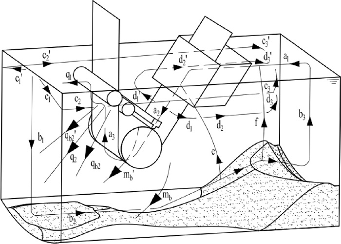
Global flow field of bottom dross.

Impact of flow field on the floor of zinc pot determines deposition morphology of bottom dross. Two main impact flows are included in the global FLBD, as displayed in Fig. 3. The thicker arrow denotes a faster flow speed. One of the main impact flows is the inverted jet produced in the area where steel strip comes to contact front support roll, as a result of their surfaces moving toward each other. The jet runs slantingly downwards to front wall (lines q₂, q_b2 and q_b2′) and impacts bottom drosses deposited in ‘front accumulation region A’. In addition, the jet is the key factor in the formation of the first circulation of FLBD stated above. Bottom drosses deposited in ‘front accumulation region A’ and ‘under roll accumulation region B’ are dispersed and heaped up in ‘back accumulation region C’. The other main impact flow is developed by the two ends of rotating sink roll where there is no belt winded around the surface. Along the tangential direction of sink roll surface, it impacts downward ‘under roll accumulation region B’ (m_b and m_b′). A couple of pits with uncovered bases (without drosses) come into being. Meanwhile, a large number of drosses accumulated in this area are scattered and join the flow field of bottom dross. Furthermore, comparisons with results of the reference¹⁷⁾ indicate that the first impact flow mentioned above does not exist in the literature due to the absent of front support roll in the model bath. The other impact flow is not given either because it is observed according to the trajectory of bottom dross as well as the location and evolution rule of impact craters. Deposition distribution of bottom dross obtained from settling of a small amount of particles cannot be used to accurately describe the dynamic accumulation of large amounts of bottom drosses.

In order to understand and display better the details of FLBD, along the width direction of zinc pot (i.e. along the X direction and parallel to the YOZ plane), a typical cross profile of FLBD in symmetry plane is shown in Fig. 4. The main characteristics of the graph are the circulation due to motions of steel strip (lines a₁→a₂→a₃→q→i→b₂→b₃). In these regions, translation of belt initially results in synchronized motions of surrounding dross-containing fluids (lines a₂ and a₃) and then has an influence on dross movement in the areas even farther (lines j, g, h, e, f and x). Surfaces of the steel strip and front support roll move toward each other (lines l and a₃). They crash in the corner and produce a strongly reversed jet flow (line q). The major part of the jet rushes slantingly downwards at front wall(line q₂). In the meantime, the rest of the jet runs horizontally or slantingly upwards to front wall (line q₁). It moves along front wall (line b₁) and combines with line q₂ into line i. The impact of jet (line i) on bottom drosses accumulated in the floor of tank results in several pits near front wall.

Fig. 4.

FLBD in symmetry plane.

Owing to the bounary effect of steel strip, ‘middle flow region II’ is separated from other zones. Motions of belt, back support roll and sink roll jointly determine the flow field of bottom dross in the area. Translation of steel sheet brings about homodromously rectilinear motions of neighbouring dross-containing liquids (lines k and p). Vacancies caused by fluids carried from snout require to be filled with other liquids nearby (lines o and w). The revolution of sink roll leads to homodromous rotations of vicinal dross-containing fluids (lines m and m₀). Line r comes into being on account of boundary effect of scraper. A zone of ‘high pressure’ where steel strip gets to contact sink roll is taken shape in virtue of their movements toward each other and then an inverted jet flow is developed (lines t and t₀). A portion of the jet containing bottom drosses merges with line o and goes into the interior of snout. Bottom drosses gather in the inner side of scraper on account of lines m₀ and t₀. In the region where the steel strip begins to depart from sink roll, a vacuum district comes out as a result of lines p and m going away from each other and is filled with surrounding dross-containing fluids (line s). Bottom drosses get together in this area due to the vacuum-filling effect except that a small number of them which touch surfaces of belt and sink roll are taken away. FLBD distributed in the contact region between steel strip and back support roll is analogous to that of sink roll. The revolve of back support roll drives adjacent bottom drosses to move along its surface (line n). Two areas of ‘high pressure’ (lines p, n and s) and ‘vacuum’ (lines p, n and u) where steel strip starts to contact and depart from back support roll are formed. Bottom drosses are always apt to heap up in the vacuum zone. Bottom drosses close to liquid level move towards steel strip (line v) owing to the effect of line u and liquid zinc taken away by outgoing belt from zinc bath.

The results also indicate that the general flow pattern inside the pot is hardly influenced by the height of bottom dross. FLBD with different heights of bottom dross exhibits the same characteristics.

4.2. Dynamic Accumulation of Bottom Dross

4.2.1. 3-D Deposition Morphology of Bottom Dross

Comparisons of 3-D deposition morphologies of bottom dross between different operation time (1st, 2nd and 3rd hour) as well as ‘initial height’ (95 mm, 75 mm, 55 mm) are illustrated in Fig. 5. The diagrams exhibit similar features of 3-D accumulation shapes for different ‘initial height’ (see (a), (b), (c)). The deposition thickness of bottom drosses in ‘front accumulation region A’ decreases successively over time. In the floor of the two impact pits near side walls, areas without drosses enlarge gradually. It leads to an outline-width reduction of deposited bottom drosses in this region. In the zone of ‘under roll accumulation region B’, the ridge becomes narrow and two craters with curved edges come to merge with pits located in ‘front accumulation region A’ as regions without drosses extend continuously. Bottom drosses which are scattered in the zones of ‘front accumulation region A’ and ‘under roll accumulation region B’ and carried by circular flows deposite toward ‘back accumulation region C’. The piling peak of bottom drosses moves close to back wall with the proceeding of running time. In addition, three typical photos (initial height 95 mm in the 3rd hour, initial height 75 mm in the 2nd hour, initial height 55 mm in the 1st hour) for deposition morphology of bottom dross are also presented in Fig. 5 (see (d)). NaCl aqueous solutions appear slight turbidity because black ABS grains are soaked and stirred in the model liquids for a long time. As can be seen from the photos, the longer the operation time is, the less particles are rolled up and the more steady the deposition morphology tends to be.

Fig. 5.

Comparison of 3-D deposition morphology of bottom dross between different operation time.

Except for the common characteristics of different dross thicknesses mentioned above, it is found from Fig. 5 that bottom dross morphologies which are deposited in the 2nd and 3rd hour for the cases of lower ‘initial height’ are very similar (see Figs. 5(b) and 5(c)). This shows that accumulation morphology with a lower ‘initial height’ approaches more quickly to be a steady state. Furthermore, at the same running time, the deposition peak for a higher ‘initial height’ is much closer to back wall (see Fig. 5(a)). The experiments also reveal that the evolution velocity of bottom dross morphology declines exponentially with the increase of operation time. The slower the evolution velocity, the less dross particles are rolled up and influence surface quality of steel strip.

4.2.2. Dynamic Characteristic and Thickness Monitoring of Bottom Dross Deposition

In order to get a comprehensive insight into dynamic deposition characteristics of bottom dross, different cross-sectional profiles of deposition morphology are given in Figs. 6, 7, 8, 9, 10 respectively. Each graph includes accumulation outlines of bottom dross for three initial heights (95 mm, 75 mm and 55 mm) as well as three operation time (1st, 2nd and 3rd hour). In these graphs, horizontal coordinates x and y represent positions of data points and are converted to dimensionless variables with the width W_t and length L_t of zinc tank separately. Vertical coordinate h denotes the thickness of bottom dross deposition and is changed to dimensionless variable with initial height H_d1=95 mm. Six positions are selected as monitoring points to measure the height of bottom dross accumulation. Locations of the six points are identical with real working conditions. Among these points, three of them are 60 mm away from front wall. Monitoring points M_1i and M_3i are at a distance of 60 mm from the left and right side wall respectively. Monitoring point M_2i is situated in the middle of the width of zinc bath. The other three monitoring points M_4i, M_5i and M_6i adjoin back wall and have the same distribution law with the first three points. Subscripts (i=1, 2, 3) of points signify thicknesses of bottom dross accumulation for three operation conditions (95 mm, 75 mm and 55 mm) separately.

Fig. 6.

A cross-sectional view of bottom dross morphology (close to front wall and with monitoring points).

Fig. 7.

A cross-sectional view of bottom dross morphology (close to back wall and with monitoring points).

Fig. 8.

A cross-sectional view of bottom dross morphology (symmetry plane along the Y axis).

Fig. 9.

A cross-sectional view of bottom dross morphology (symmetry plane along the X axis).

Fig. 10.

A cross-sectional view of bottom dross morphology (parallel to the plane YOZ and close to side wall).

Figure 6 exhibits profiles of bottom dross morphology in a section which is parallel to front wall and 60 mm apart. Outlines of bottom dross morphology for different ‘initial height’ (95 mm, 75 mm and 55 mm) display characteristics of three impact craters situated in ‘front accumulation region A’. Thickness of bottom dross deposition constantly decreases with the proceeding of running time. The width of bottom dross profile for initial height 55 mm is significantly less than the other two working conditions. From the degree of similarity between outlines of different running time, it can be deduced that heaping of bottom dross in this region has reached steady state in the third hour. Bottom dross can not be detected by monitoring points M_1i and M_3i within a short period of time, while monitoring point M_2i exactly overlaps with midpoint of the middle impact crater. The combination of the three monitoring parameters can be utilized to estimate the level of approximation between current shape and steady-state morphology.

A graph of bottom dross morphology in a plane which is parallel to back wall and 60 mm apart is provided in Fig. 7. Thicknesses of bottom dross for different working conditions (95 mm, 75 mm and 55 mm) increase over time and will be far more than its initial thickness correspondingly in the end. That the profile curves appear to be approximately horizontal lines proves synchronous accumulation of bottom dross along the width direction of zinc bath. The average value of monitoring points M_4i, M_5i and M_6i can be employed to denote the height of bottom dross deposited in ‘back accumulation region C’ and then indicates the total quantity of bottom dross accumulated in zinc pot. Moreover, the level of similarity between curves of different operation time turns out that the deposition morphology with a lower ‘initial height’ (such as 55 mm) tends to be a steady state over a relatively short period of time.

A cross-sectional view of bottom dross morphology in symmetry plane along the Y axis is shown in Fig. 8. As can be seen from the figure, for different working conditions (95 mm, 75 mm and 55 mm), the primary outlines of ridges which are located in ‘under roll accumulation region B’ take shape in the first hour. At this moment, the profile of deposition has been in a steady state (initial height 55 mm) or tends to be stable (initial height 75 mm). But in the case of initial height 95 mm, the profile of ridge shrinks and stabilizes in the next two hours. It has also been found that the heights of stable profiles for different working conditions (95 mm, 75 mm and 55 mm) approach the same value of 75 mm. This illustrates the independence between the height of stable morphology and initial height in ‘under roll accumulation region B’.

Figure 9 displays a view of bottom dross morphology in symmetry plane along the X axis. Monitering points M_2i and M_5i are situated in this symmetry plane. The figure reveals that different working conditions (95 mm, 75 mm and 55 mm) share the same characteristics. Deposition height of bottom dross in ‘front accumulation region A’ decreases and tends to be a constant value quickly. Prior to entering ‘under roll accumulation region B’, the heights of profile curves start to increase and local deposition peaks emerge. It should be noted that the height of the ridge in ‘under roll accumulation region B’ varies little and exhibits the feature of being independent of the initial height. At this point, it agrees well with the results of Fig. 8. Bottom drosses heap up in ‘back accumulation region C’ and the deposition peak continuously moves toward back wall over time. The height of the peak keeps constant during approach. The higher the initial height is, the closer the peak accesses back wall.

Figure 10 presents bottom dross morphology in a cross section which is parallel to side wall and 60 mm apart. Monitering points M_1i and M_4i are located in this plane. The figure also points out that no bottom dross stays in ‘front accumulation region A’ and ‘under roll accumulation region B’ after a short period of time. Stack heights of bottom dross in ‘back accumulation region C’ are significantly greater than initial heights correspondingly. The summit of deposited bottom drosses granually comes near to back wall over time and keeps almost the same height before arriving at back wall (coincide with Fig. 9). In the case of enough bottom dross in quantity (95 mm), the peak of accumulation can even reach back wall and a rectilinear slope is developed simultaneously.

5. Conclusions

The results are summarized as follows:

(1) The main characteristic of global FLBD is the circulation which shows that bottom drosses move from ‘front flow region I’ to ‘back flow region III’, passing three accumulation regions. This circular flow brings dispersed bottom drosses toward back wall and heaps up them in ‘back accumulation region C’.

(2) Vacuum zones appear because surfaces of the steel strip and rollers go away from each other in the contact regions between them. Bottom drosses gather in these vacuum zones as a result of filling effect which is constantly supplied by fluid nearby. Drosses escape from these regions only by the way of attachment to surfaces of the steel strip and rollers. It often occurs on one side of contact regions where the steel strip begins to depart from sink roll, back support roll and front support roll and can cause problems concerning surface quality of steel strip.

(3) There are two main impact flows to scatter bottom drosses deposited in the floor of zinc bath. One appears in the region where steel strip begins to touch front support roll and acts like a jet because surfaces of the steel strip and front support roll move toward each other. The jet rushes slantingly downwards at front wall and impacts bottom drosses deposited in ‘front accumulation region A’. The other impact flow is generated by the two ends of rotational sink roll where there is no steel strip wrapped around the surface. It ejects in the tangential direction of sink roll surface and disperses a lot of bottom drosses in ‘under roll accumulation region B’.

(4) The piling thickness of bottom drosses in ‘front accumulation region A’ declines continuously with the impact of jet. Three impact craters for symmetric distribution along front wall come into being. The middle one with a shallow bottom is the biggest. Areas without drosses in bottoms of the other two pits adjacent to side walls expand gradually and merge with craters situated in ‘under roll accumulation region B’.

(5) In the region of ‘under roll accumulation region B’, two symmetric pits with curved edges and a ridge between them are taken shape under the impact caused by two ends of sink roll. There is no bottom dross remained in the floor of the two pits. As time goes by, the pits enlarge and the ridge becomes narrow. Finally, they will tend to be a stable morphology while bottom drosses are no longer scattered. The steady-state height of the ridge is independent of the initial height of bottom dross.

(6) The leading deposition area of bottom dross is located in ‘back accumulation region C’. Acting as a wandering dune, the peak of pile-up bottom drosses approaches back wall with the proceeding of operation time. The height of the peak remains constant during approach.

(7) Bottom dross accumulations with different quantities have their own stable morphologies respectively. The evolution speed which bottom dross deposition tends to be steady-state morphology drops rapidly with the increase of running time. For bottom dross deposition in ‘front accumulation region A’ and ‘under roll accumulation region B’, the greater the distinction between current shape and stable morphology, the more dross granules are dispersed and affect surface quality of steel sheet. Three monitoring points close to front wall can be used to represent the degree of approximation between current appearance and steady-state morphology. The other three monitoring points near back wall are employed to indicate quantities of bottom dross in the zinc pot.

Acknowledgements

This work was supported by the National Natural Science Foundation of China (Grant No. 11172063, 11302046, 11502050). This support is gratefully acknowledged.

Nomenclature

Variables

C_d: drag coefficient

D: particle diameter

F_d: drag on a particle moving in liquid

Fr: Froude number

g: acceleration due to gravity

L: characteristic length

Re: Reynolds number

T: time

V: velocity

λ: scale factor

ρ: density

υ: kinematic viscosity

θ: Shields number

Subscripts

m: model

p: prototype

inc: inclusion

f: fluid

References

• 1)   J.  Li,  X. H.  Guo,  J.  Luo,  H. Y.  Li and  Y. Q.  Wang: Shock Vib., 20 (2013), 793.
• 2)   K.  Yoshiaki,  S.  Akira and  I.  Kuniyoshi: J. Jpn. Inst. Met., 71 (2007), 379.
• 3)   S. K.  Dash,  M.  Dutta and  N.  Rajesh: ISIJ Int., 45 (2005), 706.
• 4)   D. S.  Shin,  J.  Choi and  S. J.  Lee: ISIJ Int., 40 (2000), 484.
• 5)   S. J.  Lee,  S.  Kim,  M. S.  Koh and  J. H.  Chol: ISIJ Int., 42 (2002), 407.
• 6)   J.  Kurobe,  M.  Iguchi,  S.  Matsubara,  K.  Nakamoto and  Z.  Morita: ISIJ Int., 36 (1996), 438.
• 7)   Y.  Sahai and  T.  Emi: ISIJ Int., 36 (1996), 1166.
• 8)   K.  Youngjo,  S.  Bahman,  S.  Piotr,  M.  Kazuki and  S.  Du: Metall. Mater. Trans. B, 42 (2011), 522.
• 9)   M. J.  Zhang,  H. Z.  Gu,  A.  Huang,  H. X.  Zhu and  C. J.  Deng: J. Min. Metall. B, 47 (2011), 37.
• 10)   S. X.  Liu,  X. M.  Yang,  L.  Du,  L.  Li and  C. Z.  Liu: ISIJ Int., 48 (2008), 1712.
• 11)   N. J.  Themelis,  P.  Tarassoff and  J.  Szekely: Trans. Metall. Soc. AIME, 245 (1969), 1425.
• 12)   A. S. C.  Marco,  C.  Branco and  K.  Schwerdtfeger: Metall. Mater. Trans. B, 27 (1996), 231.
• 13)   K.  Krishnapisharody and  G. A.  Irons: Metall. Mater. Trans. B, 44 (2013), 1486.
• 14)   K.  Krishnapisharody and  G. A.  Irons: ISIJ Int., 50 (2010), 1413.
• 15)   J.  Kurobe and  M.  Iguchi: Sci. Technol. Adv. Mater., 1 (2000), 251.
• 16)   J.  Kurobe and  M.  Iguchi: Mater. Trans., 44 (2003), 1429.
• 17)   J.  Kurobe and  M.  Iguchi: Mater. Trans., 44 (2003), 885.
• 18)   D.  Hryb,  M.  Cardozo,  S.  Ferro and  M.  Goldschmit: Int. Commun. Heat Mass Transf., 36 (2009), 451.
• 19)   C. F. M.  Coimbra and  R. H.  Rangel: Fluid Mech., 370 (1998), 53.
• 20)   R. H.  Perry and  D. W.  Green: Perry’s Chemical Engineers’ Handbook, 8th ed., McGraw-Hill, New York, (2007), 56.
• 21)   K. E. K.  Abderrezzak,  A.  Die. Moran, E. Mosselman, J.-P. Bouchard, H. Habersack and D. Aelbrecht: J. Hydro-Environ. Res., 8 (2014), 95.
• 22)   R. K.  Sinnott: Coulson & Richardson’s Chemical Engineering, Vol. 6, Chemical Engineering Design, 4th ed., Butterworth-Heinemann, Oxford, (2005), 73.