Prediction of the Temperature Distribution and Microstructure in the HAZ of SA508Gr4 Reactor Pressure Vessel Steel

Abstract

SA508Gr4 is a newly developed steel for reactor pressure vessel and its behavior data is rare, especially its welding characters attract researchers and industries attention. In this paper, a finite element method (FEM) is employed to investigate the thermal process and phase transformation process of arc welding of SA508Gr4 steel, where a body heat source model and element birth and death technique were used in this simulation process. This study focuses on the effect of peak temperature (t_m) and cooling rate (t_8/5) on microstructural transformation in HAZ, which is to be overcome by combining SH-CCT diagram with numerical thermal cycle curves. Through conversion of thermal cycle data into microstructural information, it is found that the quenched zone is developed rapidly whose width is 1560 µm, while the inter-critical HAZ region is three times smaller than the quenched zone dimension, which is 450 µm. Post weld heat treatment was suggested to be adopted for improving the property of HAZ. In addition, the metallographic analysis confirms the expected microstructural evolutions. The microstructure is martensite (M) + some bainite (B) and the microhardness is between 429 HV and 432 HV.

1. Introduction

Reactor pressure vessel (RPV) has been built that was designed and constructed by SA508Gr3 forging and SA533B steel plates materials in most countries to date. PRV with an increasing trend in direction of large-scale and integrated development, it is difficult to ensure the homogeneity of microstructure and stability of performance of ultra-thick plate on the cross section. However, increasing the thickness of plates may cause a great problem for welding. Many researchers have tried to improve the mechanical properties of PRV material by controlling the chemical composition of conventional RPV steels. SA508Gr4 steel, as a new generation RPV steel, in which Ni, Cr contents is larger and Mn contents is lower than typical steels, may be a promising RPV material with higher strength and stronger resistance to irradiation embrittlement from its tempered martensitic microstructure.^1,2)

As a weak link in the RPV, the brittle fracture, creep-deformation, corrosion cracking, fatigue failure and etc. of welding heat affected zone (HAZ) may be the most important reason for leading to security incidents and failure. For SA508Gr4 alloy steel, the appearance of brittle cracks in the HAZ results in premature structure failure during extended service. Lee et al.³⁾ of Korea Institute of Science of Technology (KIST) has a number of achievements in exploring the mechanical strength for SA508Gr4 steel, but experimental test alone can hardly predict about all properties on active service of welded joint. Now accurate predication can be realized for welding deformation, welding stress and welded joint microstructures by using finite element method (FEM), it also provides reference to prevent cracking or buckling, which is caused by local production internal structure damage.^4,5,6) It is necessary to study the effects of welding parameters on the quality of welding of SA508Gr4 steel in order to achieve the optimum weldability.

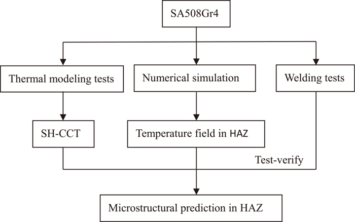
In this paper, FEM is used to establish the model of the double-V groove arc welding of SA508Gr4 steel to calculate the temperature field, of which applied the key parts of nuclear pressure vessel steel. The effects of the peak temperature t_m and cooling rate t_8/5 (the welding thermal simulation cooling time between 800 and 500°C) of the thermal cycle on phase transformation are systematically investigated. Based on the above researches, the microstructure of HAZ for SA508Gr4 steel can be predicted by combining the Simulated HAZ continuous cooling transformation (SH-CCT) diagram with numerical simulation thermal cycle curves. The test flow chart is shown in Fig. 1.

Fig. 1.

Flow chart.

2. Welding Test and FEM

2.1. Experimental Material

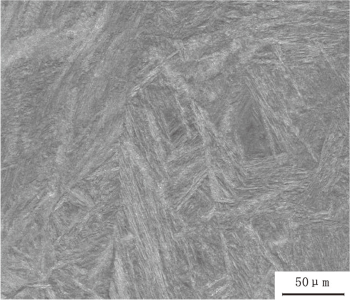
The material used in this study is hot-rolled SA508Gr4 RPV steel, and the specific chemical components with different alloying element contents based on the composition range of American standard ASME spec. are given in Table 1. SEM image of the base material is shown in Fig. 2, the predominant microstructures are tempered martensite (TM) with embedded fine carbides. The M is formed along the austenite grain boundary and a large amount of Cr–C compounds dispersed due to the substrate with high Cr, which is coincided basically with the carbide microstructures mentioned in the literature.⁷⁾ Its hardness is up to 412 HV, the solidus temperature is measured by using STA449C machine: T_L=1498.7°C, and critical temperatures are measured by using L78 Rita Quenching and Deformation Dilatometer (shown in Fig. 3): A_c1=662.7°C, A_c3=796°C.

Table 1. Chemical composition of the base metal and filler wire (wt, %).

	C	Mn	P	S	Cr	Ni	Si	Al	Mo	Fe
ASME spec.	≤0.23	0.2–0.4	≤0.02	≤0.015	1.5–2.9	2.8–3.9	≤0.3	–	0.4–0.6	Bal.
Specimens	0.12	0.36	0.0054	0.0034	2.40	3.64	0.096	0.016	0.60	Bal.
J857CrNi	0.056	1.65	0.020	0.015	1.55	2.60	0.29	–	0.56	Bal.

Fig. 2.

SEM micrograph of the tested materials.

Fig. 3.

L78 Rita Quenching and Deformation Dilatometer. (Online version in color.)

2.2. Welding Preheating Temperature

In consideration of the effects of individual elements on steel hardening tendency, especially the role of the C,⁸⁾ the cold crack sensitivity is evaluated indirectly by calculating the carbon equivalent (CE), the formula of CE is employed to judge the hardening tendency that recommended by the IIW:⁹⁾   

$$CE=\mathrm{C}+\frac{\mathrm{M}\mathrm{n}}{6}+\frac{\mathrm{C}\mathrm{r}+\mathrm{M}\mathrm{o}+\mathrm{V}}{5}+\frac{\mathrm{C}\mathrm{u}+\mathrm{N}\mathrm{i}}{15}(\%)$$(1)

In general, CE≤0.4% is considered to meet the basic demands of weldability. The calculations value of CE is 1.023% according to Eq. (1) for the application of the RPV steel, which indicates that it is unable to suffice for the demands above mentioned. High hardening tendency and crack susceptibility of SA508Gr4 steel are the main factors that make it difficult to achieve good welds as welding thick plate. The welding process should be strictly controlled in arc welding.

Alloy elements of SA508Gr4 steel such as Mn, Ni, Mo in total content is about 7%, which belongs to the category of low carbon alloy steel, according to cold crack sensitivity index (P_cm) and cold-cracking susceptibility (P_c) formula:¹⁰⁾   

$$P_{\mathrm{c}\mathrm{m}}=\mathrm{C}+\frac{\mathrm{S}\mathrm{i}}{30}+\frac{\mathrm{M}\mathrm{n}+\mathrm{C}\mathrm{u}+\mathrm{C}\mathrm{r}}{20}+\frac{\mathrm{N}\mathrm{i}}{60}+\frac{\mathrm{M}\mathrm{o}}{15}+\frac{\mathrm{V}}{10}+5\mathrm{B} (\%)$$(2)

  

$$P_{\mathrm{c}}=P_{\mathrm{c}\mathrm{m}}+\frac{\left[\mathrm{H}\right]}{60}+\frac{\sigma }{600}$$(3)

  

$$T_0=1\mathrm{\hspace{0.17em} }440P_{\mathrm{c}}-392$$(4)

where [H] stands for the content of hydrogen diffusion [H]=2.0 ml/100 g, from their actual thickness σ to the reference thickness σ=12 mm, T₀ is the preheating temperature for avoiding cold cracking. The calculations show that SA508Gr4 steel has high hardening tendency and cold-cracking susceptibility (P_c = 0.407%) during welding with preheating temperature of 202°C or above as a large restraint.

2.3. Welding Process

The SA508Gr4 high-tensile steel plates with dimension of 300×100×12 mm are used in experiments, which the weld length is 100 mm at the approximate middle section of the plates. Manual arc welding tests are conducted on steel, and a butt joint configuration is used with the metal core of J857CrNi welding electrode as filler metal, their chemical compositions are shown in Table 1. The plate needs double-V symmetry groove (angle=60°). The whole weld process consists of 2 passes all together, including 1 pass in the upside and downside of plate individually. The welding parameters: welding current I=120 A, welding voltage U=30 V, welding speed v=2.3−2.4 mm•s⁻¹, heat input Q=15−16 kJ•cm⁻¹, determine the preheating temperature is 202°C based on the calculations of cold-cracking susceptibility, so is the lower inter-pass temperature. The welding thermal efficiency, denoted η, is assumed as 60%.

The thermal cycles of welding plates is performed by using XSR30 paperless recorder and Chromel-Alumel thermocouples whose withstanding temperatures as large as 1200°C. The positioning of the thermocouples is decided close to the melted zone where large temperature gradients are expected.

2.4. Formulation and Grid Structure

The welding simulation has made a large progress in recent years. It allows the understanding of complex interactions during welding heating and cooling and thereby a more targeted optimization of the joint microstructure.

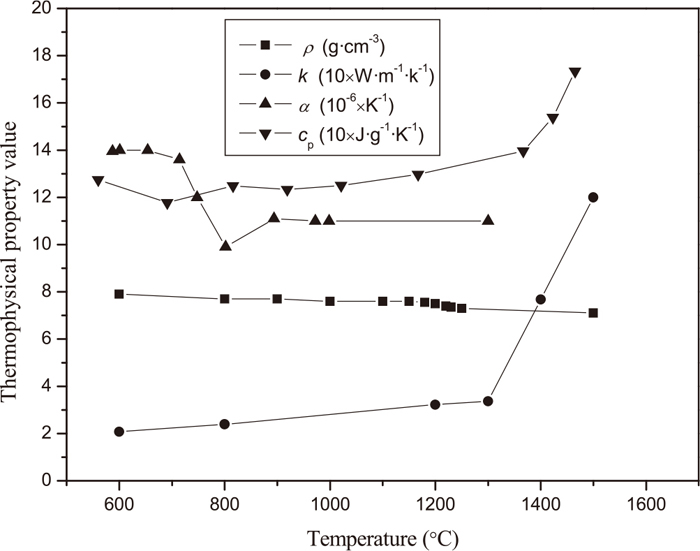
The simulation of welding process is conducted by ANSYS software. In simulation model, it is necessary that it has correct material properties. The weld material had the properties that before the temperature are lower than the steel melting point and its material properties are changed after temperature exceeded steel melting point. The thermophysical properties of SA508Gr4 alloy steel varying with temperature are shown in Fig. 4.¹¹⁾

Fig. 4.

Material properties of SA508Gr4 steel.

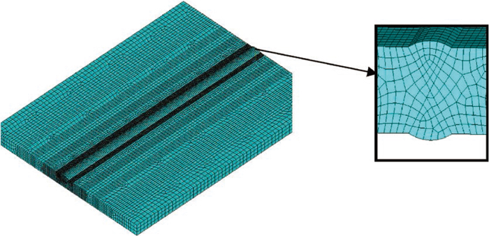
A full three-dimensional FEM of the specimen is developed and the necessary correlations are implemented to make the model as accurately as possible, Fig. 5 shows the initial grid employed for thermal analysis. A variable spacing grid system with a fine grid near the heat source and a course grid away from the heat source has been used for model the heat transferring. The computational domain consists of 85380 elements, and the ambient temperature was set at 25°C. All of the materials are assumed to be isotropic and the filler metal has the same material properties as SA508Gr4 base metal. The course of stuffing, melting, freezing of metal in welding seam is simulated successfully with the birth-death element method,¹²⁾ and a body heat source model is used for simulating the welding heat source of the steel plate. The grids of each pass are divided into independent units, and they are defined as dead unit before welding. The units in weld zone are activated one by one during welding process.

Fig. 5.

Finite element grid generation. (Online version in color.)

Boundary conditions must be defined by including prescribed temperature (first type boundary condition) and prescribed convection heat transfer coefficient (third type boundary condition). The approximate solution of the nonlinear differential equation in thermodynamics of the each control volume within the domain is accomplished by a variational method and finite element method, the nonlinear three-dimensional transient heat conduct equation has the following form:¹³⁾   

$$\frac{\partial \left(K_x\frac{\partial \theta }{\partial x}\right)}{\partial x}+\frac{\partial \left(K_y\frac{\partial \theta }{\partial y}\right)}{\partial y}+\frac{\partial \left(K_z\frac{\partial \theta }{\partial z}\right)}{\partial z}+Q_b=0$$(5)

Where Q_b stands for heat generation rate per unit volume, K_x, K_y, K_z is the thermal conductivity in three directions for X, Y and Z, respectively. The method of Newton-Raphson is used in solving process that the convergent speed and computing precision are excellent.¹⁴⁾

3. Simulation Results

3.1. Temperature Field

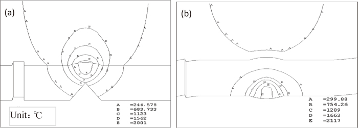
Welding simulation is in the same condition as experiments. Figures 6(a)–6(d) show the calculated temperature distribution of four stages during the welding process which are the steel plates after preheating, the first pass weld, the second pass weld and 5000 s cooldown after welding. The corner regions with two-dimensional heat dissipation is fast, which leads to the corner regions temperature is slightly below the other regions, as shown in Fig. 6(a). Quasi-steady state of temperature distribution is obtained after arc initiating. In Figs. 6(b), 6(c), a welding heat source, form and maintain oval-shaped temperature gradient. It is apparent that the symmetric temperature distribution observed at the weld center line to keep the maximum temperature above 2352°C at first pass, the second pass above 2229°C. An approximately uniform temperature field is provided after welding 5000 s as shown in Fig. 6(d).

Fig. 6.

Comparison of temperature distribution at different time. (a) Welding preheat; (b) 68 s Welding; (c) 350 s Welding; (d) 5444 s Welding. (Online version in color.)

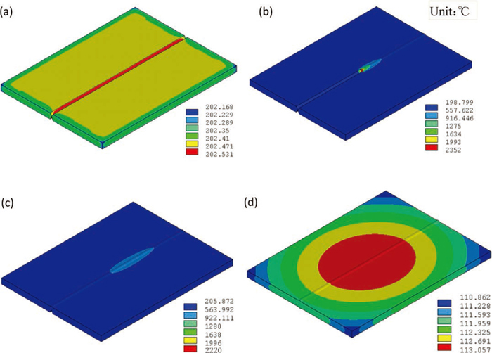
Figure 7 shows the transient temperature isopleths on the cross-section of welding heat source. For the case of the model, the temperature of line E and D is above T_L, while assumed as the welding heat source, and line A, B, C assumed as the temperature isopleths of the base metal. The arc welding pool with ideal shapes is obtained, and the predicted ones are presented. The temperature gradient is not as large as heating during cooling, and approximating range of temperature profile exhibits clearly which represents liquid-solid phase transformation. It follows the laws of heat transfer that the magnitude of temperature change depends on the distance from the welding line.¹⁵⁾

Fig. 7.

Temperature isopleths of calculating locations in welded joint. (a) 68 s Welding; (b) 350 s Welding.

3.2. Analysis and Validation of Thermal Process

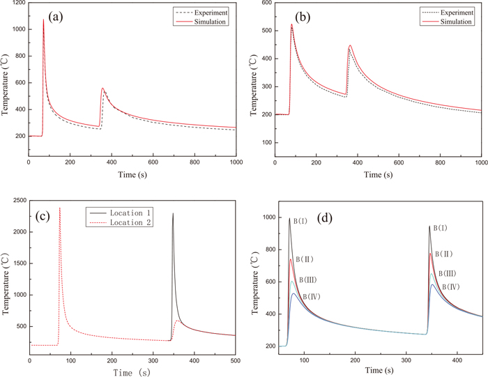
The distribution of measuring locations is shown in Fig. 8. Figures 9(a) and 9(b) presents the validation of numerical model based on comparison between experimental and simulation thermal cycles at two different positions associated to thermocouples location 3 and 4 in Fig. 8. The peak temperature of simulation results are both higher than the experimental results. The reason for the difference may be the neglect of the influence of fluid motion on heat transfer mechanism. The difference between peak temperature values is less than 9.5% for location 3 and 2% for location 4. On the other hand, the cooling rate t_8/5 of numerical is 15.7 s for location 3, experiment is 14.5 s, an 8.3% difference. Similarly, the mean relative deviations of numerical and experiment are less than 10% for location 4. Therefore, the whole evolution trend of experimental temperature agrees approximately with that of calculated temperature, and the presented model and conclusion are proved to be correct.

Fig. 8.

The arrangement of temperature measurement locations. (Online version in color.)

Fig. 9.

Characteristic welding thermal cycle curves. (a) location 3; (b) location 4; (c) location 1, 2; (d) path B. (Online version in color.)

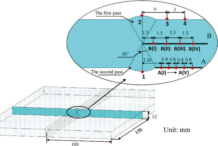
The thermal cycles are predicted at a particular position corresponding to location 1 and 2 in Fig. 8, which are located on the surface of welding passes. Figure 9(c) shows the calculated results of welding thermal cycle at location 1 and location 2. The metal is heated to T_m =2390°C at a rate of 287°C/s at location 2, which stayed in high temperature area (t_H above 1100°C) for 9.13 s and subsequence cooled to 800°C at a rate of 147°C/s, eventually to 500°C under a cooling time for 14.5 s. Due to the rapid heating and cooling rates applied in the welding process, the materials of these positions undergo a non-equilibrium phase transformation. It is reheated to 592°C same as temper process during the second pass coming.

The locations where it is difficult to measure the welding thermal cycle on the path B in Fig. 8 are named of B(I), B(II), B(III) and B(IV) from left to right. Figure 9(d) presents the peak temperature of thermal cycles varied with different positions of weld joint interface during arc welding by numerical simulation. All attempted positions produce the same overall shape of the thermal cycle including a sharp increase in temperature followed by a smoother tail corresponding to the cooling stage. The sharp profile exhibited by B (I) (T_m=996°C, t_8/5=18.11 s) indicates a close position to the welding seam whereas the most eccentric position B (IV) produces a rounded peak. The position B (I) and B (II) can be considered as belonging to HAZ. Those results confirm what is reported in the paper about welding thermal cycles, the T_m and t_8/5 will clearly change associated with the different positions of welding seam, which means that the T_m and t_8/5 rapid change will influence on the microstructure changes of HAZ.

4. Microstructural Predictions and Analysis in HAZ

4.1. Predict the Extent of the HAZ

The extent of HAZ increasing with the heat input of the welding process is undertaken to evaluate the extent of the risk zones introduced earlier. The above content illustrates that the temperature appears two peaks. The second heat cycle is induced by rear pass and equal to post-heat action to the fore pass. Similarly, fore pass induces preheat action to the rear pass.¹⁶⁾ The double-peak character of arc welding temperature will improve weld microstructure and alleviate the cold crack. But the rear pass activity may cause abnormal grain growth to the fore pass in HAZ, so the last heat cycle is selected for study to avoid affecting the predicted microstructure. The HAZ of the steel with hardenability to be divided into two sub-regions: quenching HAZ region (Q-HAZ) and inter-critical HAZ region (IC-HAZ).

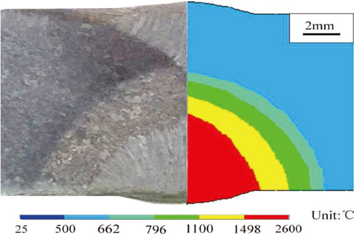
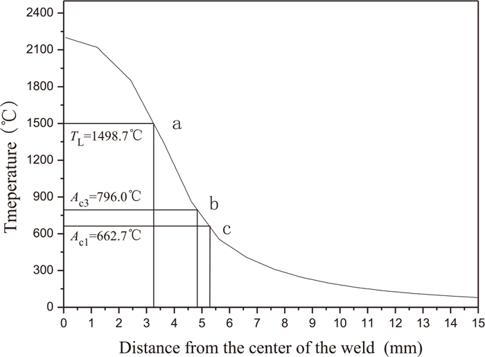
The widths of each phase are critical to predict damage evolution and failure after welding. Figure 10 shows the transverse transient temperature distribution on the surface of path A (in Fig. 8) during the second arc pass approaching by numerical simulation, which illustrates that the transient temperature is decreased significantly with distance increasing from welding heat source and the sizes of widths of HAZ is temperature-dependent. The fusion line is formed during the subsequent cooling from peak temperature (T_m=2299°C) to the solidus temperature (Fig. 10 point a) and begins to calculate the domain sizes of HAZ. The outcome is that the domain sizes of Q-HAZ is 1560 μm, which is approximately 77% of the total HAZ width, and the formation temperature range is from T_L to A_c3 (part ab); IC-HAZ with a narrow width of 450 μm in which peak temperature is between A_c1 and A_c3 (part bc), per region that put together to make up the total HAZ width of 2010 μm. Above phenomenon can be explained as follows, firstly, the temperature gradient of the Q-HAZ of arc welding is bigger than that of IC-HAZ because of the distance from heat sources. Secondly, the total heat loss in IC-HAZ is lower because of thermal accumulation. The contours of the simulated result is in accordance with the HAZ micrograph of a mid-thickness plane shown in Fig. 11, some evidence can be seen of edge-width in both IC-HAZ and fusion line. Hence if the number of node is enough in the HAZ, thermal history of microstructure in HAZ can be predicted by FEM in order to identify the range of HAZ microstructure.

Fig. 10.

Transverse transient temperature distribution of path A.

Fig. 11.

Weld pool shape comparison experimental (left) and simulation prediction (right). (Online version in color.)

4.2. Microstructure-property Prediction and Analysis in HAZ

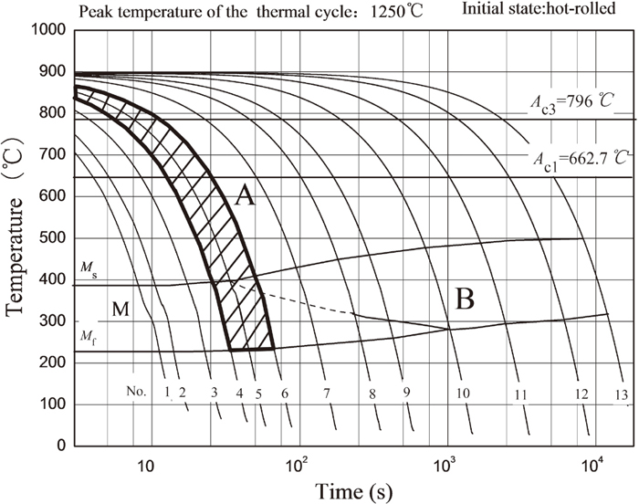
The phase transformation temperatures of SA508Gr4 under rapid heating rates are measured by welding thermo-simulated test (L78 Rita Quenching and Deformation Dilatometer). The Simulated HAZ continuous cooling transformation (SH-CCT) curves of SA508Gr4 steel are obtained, as indicated in Fig. 12, and Table 2 can be referred for more detailed information. It can be roughly divided into martensite (M) and some bainite (B) transformation regions. The t_8/5 critical cooling time of the above two phase transition is 18 s and 520 s respectively.

Fig. 12.

The SH-CCT diagram of SA508Gr4 steel.

Table 2. Cooling rate dependent Microstructure transformation percentages and microhardness value of welding.

No.	Cooling rate (°C/s)	t8/5/s	Microhardness/HV	Average volume fractions of microstructure (%)	Critical cooling time (s)
1	65	4.6	454	M100	t’b=18
2	50	6	441	M100
3	30	10	441	M100
4	20	15	429	M100
5	15	20	432	B2 M98
6	10	30	431	B10 M90
7	5	60	423	B20 M80
8	2.5	120	433	B73 M27
9	1.5	200	423	B90 M10
10	0.6	500	411	B95 M5
11	0.25	1200	401	B100	t’m=520
12	0.1	3000	371	B100
13	0.05	6000	352	B100

The thermal cycle curves of five nodes on path A by the numerical simulation is shown in Fig. 13 where the peak temperature is below T_L, by the name of A(I), A(II), A(III), A(IV) and A(V) from left to right. The distance from center to A(I) is 3.2 mm, which was given according to Fig. 10 (the distance from the center to T_L). The processes for microstructure-property prediction are as follow: Firstly, the HAZ is segmented into different regions. In Fig. 13, the curve A(I), A(II) and A(III) belong to the Q-HAZ while A(IV) belongs to IC-HAZ and determined from independent peak temperature T_m; secondly, the measured t_8/5 between A(I) and A(III) is within 19.2–23 s; finally, the time is in the scope of t_8/5 between No.4 and No.6 according to the Table 2, and is marked in SH-CCT where the phase transformation will take place (The shadow zone in Fig. 12). The microstructures of HAZ have been predicted to be M and M+B, and the microhardness fluctuates in the range between 429 HV and 432 HV.

Fig. 13.

Welding thermal cycle for path A.

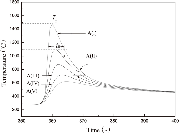
The microstructures of a welded joint are typical not uniform. Different areas of the steel will experience different thermal processes, which lead to the evolution of a more complex microstructure. The SEM micrographs of etched welded joint are explored in Fig. 14. A zoom-out view shows the separation between domains, allowing for the definition of a clear fusion line. Figure 14(a) is the typical SEM view of Q-HAZ and weld metal (WM) for second pass. The microstructures of WM contain interlaced needle-like structures in nearby Q-HAZ where to form martensite with a large number of lath bundles along austenite crystal boundary. The growth behavior of grain during arc welding is the function of temperature and time. The growth equation of austenite grain in HAZ is derived from the Arrhneoius formula¹⁷⁾ at equilibrium heated as follow:   

$${\mathrm{D}}^{1/\mathrm{n}}-{\mathrm{D}}_0^{1/\mathrm{n}}=\mathrm{K}{\int }^{\mathrm{t}}exp(-\mathrm{Q}/\mathrm{R}\mathrm{T}(\mathrm{t}))\mathrm{d}\mathrm{t}$$(6)

where D₀ is the initial grain size in HAZ, D is the average grain size in HAZ, Q is the grain growth activation energy, T(t) is the equation of welding thermal cycle, n is exponential of grain growth processes (temperature dependent), K is constant and R is gas constant. Previous research has shown that^18,19,20) the peak temperature (T_m in Fig. 13), the high temperatures residence times (t_H in Fig. 13) and cooling rate (α in Fig. 13) in thermal cycle based on the R. Senal equation,²¹⁾ which has significantly effect on the grain size and mechanical properties. Numerical thermal cycle shows T_m maximum at location A (I) as large as 1480°C, in addition, t_H=4.8 s and t_8/5=19.2 s, the microstructure as shown in Fig. 14(b). The microstructure of Q-HAZ close to the WM which include the new grain forms toward the crystal boundary and the initial grain growth. There is a significant tendency of grain growth at Q-HAZ as a consequence of the heat transfer in HAZ, and the grain size increased from 23 μm (base metal) to 100 μm. Figure 14(c) shows the microstructure of object tag in Fig. 14(b). The quenched M is formed in the area of Q-HAZ due to a larger driving force for M when t_8/5=19.2 s. There are M-A constituents with a small size formed in the matrix of M, which consists of carbon-enriched, as indicated by the arrow shown. It does illustrate the time for atoms of C and other alloy elements to diffuse are not sufficient. M-A constituents, are usually regarded as crack initiators in the local brittle zone because of their higher hardness and brittleness compared with the matrix microstructure. The existence of M-A and a large width of Q-HAZ will lead to the toughness decrease.^22,23) Therefore, the microstructure in this region is distributed more nonuniform than the other zones. Post weld heat treatment is suggested to be adopted for improving the property of HAZ.

Fig. 14.

The microstructure of the HAZ. (a) The SEM view of fusion line; (b) the microstructure of location A(I); (c) The microstructural of inner contour line in Fig. 13 (b); (d) The microstructure of location A(III).

Figure 14(d) shows the microstructure approaching location A(III), which near the border of Q-HAZ and IC-HAZ. The peak temperature of the microstructure at A (III) is 872°C and the cooling t_8/5 is 23 s, indicating a slower cooling stage than A (I). The carbon atom in the austenite can linger for a long time and diffuse toward the area, but the time is not enough. The M and some B with embedded fine carbide are obtained, as indicated by the arrow shown. The carbide, including undissolved carbide in tempered martensite (the base metal) and new carbide precipitate is formed under slower cooling rate. B transformation belonged to diffusion transformation, it can be considered that the diffusion transformation is occurred with the average volume fraction of B is above 2% according to Table 2 and Fig. 14(d). The microstructure of actual welded joint in Q-HAZ is M + B, which is in fair agreement with predicted result.

5. Conclusions

The microstructure of the HAZ of reactor pressure vessel SA508Gr4 steel is properly predicted by using numerical simulation with thermal simulation (SH-CCT) methods. The following conclusions are drawn based on the results of this study:

(1) The simulated values agree well with observed values of welding thermal cycle curve which show that the numerical model deviates by less 10%. This evidence supported by microstructural analysis in HAZ, thermal cycle curves analysis and domain sizes analysis of the welded joint.

(2) A good approximation of the domain sizes of HAZ is predicted at the heat input as large as 15–16 kJ/cm. At the centre area exposed to the heat source, the quenching HAZ region width is approximately 1560 μm, while inter-critical HAZ region with a narrow width of 450 μm, per region that puts together to make up the total HAZ width of 2010 μm.

(3) Predicted microstructure is martensite+ a little bainite, and the microhardness between 429 HV and 432 HV in the quenching HAZ region. There is the M-A constituents with a small size formed in the matrix of M when t_8/5=19.2 s. The diffusion transformation with embedded fine carbide is occurred when t_8/5=23 s.

Acknowledgement

This work was supported by Important National Science & Technology Specific Projects. (No. 2009ZX04014-064-05) and Scientific research project of Colleges and Universities in Inner Mongolia Autonomous Region (No. NJ10092).

References

• 1)   W.  Yang: Nuclear Reactor Material, Atomic Energy Press, Beijing, (2000), 12.
• 2)   Y.  Nishiyama,  K.  Onizawa,  M.  Suzuki,  J. W.  Anderegg,  Y.  Nagai,  T.  Toyama,  M.  Hasegawa and  J.  Kameda: Acta Mater., 56 (2008), 4510.
• 3)   K. H.  Lee,  S. G.  Park,  M. C.  Kim,  B. S.  Lee and  D. M.  Wee: Mater. Sci. Eng. A, 529 (2011), 156.
• 4)   D.  Deng,  H.  Murakawa and  W.  Liang: Comput. Method. Appl. Mech. Eng., 196 (2007), 4613.
• 5)   A.  Capriccioli and  P.  Frosi: Fusion Eng. Des., 84 (2009), 546.
• 6)   J.  Fanchi: Energy in the 21st century, World Scientific Publishing Company, Hackensack, (2011), 23.
• 7)   K. H.  Lee,  M. C.  Kim,  B. S.  Lee and  D. M.  Wee: J. Nucl. Mater., 403 (2010), 68.
• 8)   H. K.  Sung,  Y. S.  Sang,  B.  Hwang,  G. L.  Chang,  N. J.  Kim and  S.  Lee: Mater. Sci. Eng. A, 530 (2011), 530.
• 9)   R. G.  Faulkner,  S.  Song,  P. E. J.  Flewitt,  M.  Victoria and  P.  Marmy: J. Nucl. Mater., 255 (1998), 189.
• 10)   Y.  Ito and  K.  Bessyo: Weldability Formula of High Strength Steels Related to Heat Affected Zone Cracking, IIW Document, international institute of welding, France, (1968), No. IX-576-68.
• 11)   Q.  Bai: M. Sc. thesis, Inner Mongolia University of Science and Technology, (2015), http://epub.cnki.net/kns/brief/default_result.aspx, (accessed 2015-05-30).
• 12)   L.  Wang,  Y.  Wang,  X. G.  Sun,  J. Q.  He,  Z. Y.  Pan and  C. H.  Wang: Comput. Mater. Sci., 53 (2012), 117.
• 13)   X.  Jin,  L.  Li and  Y.  Zhang: Int. J. Heat Mass Transf., 46 (2003), 15.
• 14)   H. W.  Hesselbarth and  I. R.  Göbel: Acta Metall. Mater., 39 (1991), 2135.
• 15)   C. S.  Wu: Welding Thermal Precesses and Weld Pool Behaviors, China Machine Press, Beijing, (2007), 53.
• 16)   H. J.  Zhang,  G. J.  Zhang,  C. B.  Cai,  H. M.  Gao and  L.  Wu: Mater. Sci. Eng. A, 499 (2009), 309.
• 17)   I.  Andersen,  Ø.  Grong and  N.  Ryum: Acta Metall. Mater., 43 (1995), 2689.
• 18)   S.  Deda and  L.  Jiajun: High Temperature Metallography, Tianjin University Press, Tianjin, China, (2007), 80.
• 19)   D. M.  Rodrigues,  L. F.  Menezes and  A.  Loureiro: Eng. Fract. Mech., 71 (2004), 2053.
• 20)  Q. Z. xia, T. Z. ling, D. Z. yu, H. C. hong, Z. X. wu, B. Yang: Trans. China Weld. Inst., 21 (2000), 90.
• 21)   M. F.  Ashby and  K. E.  Easterling: Acta Metall., 30 (1982), 1969.
• 22)   R.  Ding and  Z. X.  Guo: Mater. Sci. Eng. A, 365 (2004), 172.
• 23)   L.  Lan,  C.  Qiu,  H.  Song and  D.  Zhao: Mater. Lett., 125 (2014), 86.