Temperature Control Technology by Finite Difference Scheme with Thickness Unequally Partitioned Method in Gradient Temperature Rolling Process

Abstract

In order to solve the problem of low the computational speed in gradient temperature rolling (GTR) process and guarantee the accuracy of temperature distribution in thickness direction, temperature control technology by finite difference scheme with thickness unequally partitioned method was investigated. The thickness partitioned method is adopted by means of equidistance logarithmic value for thickness, which causes the distance of two neighboring nodes to be larger as thickness increasing and gets the effect of more detailed grid on surface and rough grid in the core. Finite difference scheme was used to study the formation law of the temperature field which considers effect of oxide scale thickness in thickness direction, then temperature distributed regularity with different heat transfer coefficients in thickness direction of plate was obtained. The temperature distributions of gradient temperature rolling process is calculated while rolling procedure running, temperature gradient change rules over time with certain water jet pressure as well as temperature gradient change rules with different water jet pressures are studied. The industrial testing result illustrates that calculated rolling force reference and rolling torque reference are slightly larger than neighboring values by about 10% when gradient temperature rolling mode is used in pass 1, pass 3, pass 5 and pass 7. From comparison of measured temperature and calculated temperature, it indicates that prediction difference can be controlled with ±5°C when node number equals to 16 with half thickness and deviation of calculated force and measured force can be controlled with ± 4.0%.

1. Introduction

Ultra-heavy plate is widely used in construction machinery, ship building, ocean engineering and pressure vessels, etc. Laminar cooling processes is used in hot-rolled plate manufactory, since it is crucial to the quality of production except of alloying elements and the mechanical properties of plate are directly determined by the cooling curve and finished cooling temperature of plate.^1,2,3,4,5) Han and Lee et al.⁶⁾ use the thermo dynamic model to estimate the spatial distribution of strip temperature, but the measurements are not used to correct the dynamic model’s outputs. In order to precisely estimate the spatial distribution of strip transient temperature, Serajzadeh and Karimi et al.⁷⁾ use measurement signals to correct the results estimated only by model, and then to restrain the disturbances. Fortunately, due to the rough production environment including high temperatures, water vapor and vibrations in ultra-heavy plate rolling process, measurements for feedback control like hot strip rolling⁸⁾ are difficult or impossible, in particular for the full length of the produced is too short. More importantly, the cooling capacity of laminar cooling processes is not enough to control the center part of ultra-heavy plate, in which the cooling rate is low and results in the uneven heat transfer.

In order to improve the microstructure property of the plate center as well as the deformation uniformity in thickness direction, a rolling technology with large deformation resistance gradient is used by means of rapidly cooling the work piece surface, which causes the deformation going deep into the center part of the ultra-heavy plate and increasing the quality of the center part. Yu et al.⁹⁾ developed a novel gradient temperature rolling (GTR) process, in which the temperature field, strain, and stress of the rolling piece were calculated by finite element modeling and the plate rolled under gradient temperature conditions had excellent mechanical properties. Zhang et al.¹⁰⁾ use finite element method to explore the variation of widthwise metal flow in temperature gradient rolling, by which the metal deformation in width direction has to be controlled to ensure that the side-surface shape of plate is close to flatness so as to decrease widthwise trimming loss of heavy plate. While finite element simulations can deliver the required level of detail, computations typically take from several minutes to hours. This is too slow to be of practical use in online process control.

Model predictive control is naturally a good method to take this task since it could directly treat with measurable disturbances, and has been widely recognized as a practical control technology with high performance.^10,11,12) It is well known that the finite difference method is a powerful numerical analysis tool for solving temperature on-line controlling.^13,14,15) The grid division of traditional finite difference method is evenly distributed. However, in gradient temperature rolling process, the temperature of plate surface is much smaller than plate core part. So more detailed grid is needed to guarantee the accuracy of temperature distribution in thickness direction, but which will significantly slow down the computational speed and influence the effectiveness in online process control. In this paper, a thickness unequally partitioned method is used to divide mesh gradually detailed from center to surface, and the distribution of grid satisfies exponential distribution law.

2. Experimental Facilities

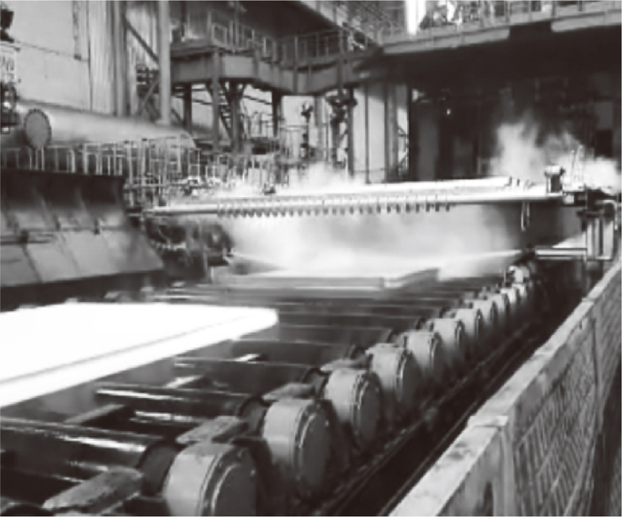
A schematic view of the gradient temperature rolling facility can be seen in Fig. 1. The facility consists of a four-high mill, a top water tank, a bottom water tank, flow control valves, water pump, top planar jet, bottom jets, two radiant pyrometers installed in upstream and downstream of stand and two blow equipment installed upstream and downstream of stand.

Fig. 1.

Schematic view of the gradient temperature rolling facility.

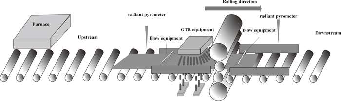
The heat rolled E355DD is adopted as the steel plate, whose mass fraction of chemical composition is: 0.17C, 0.45Si, 1.52Mn, 0.05Nb, 0.05Mo, 0.17Ti, the slab size is 300 mm×1800 mm×2800 mm, the target size is 75 mm × 2600 mm×7269 mm. The density of the steel is assumed density is 7860 kg/m³ at 20°C. Thermo-physical properties for AISI 304L is shown as Table 1. The roller surface length of four-high mill is 3500 mm, the diameter of work roller is 950 mm, and Maximum rolling force is 70000 kN, Maximum motor power is 7000 kW. The GTR equipment is developed by Northeasten Univercity of China and is installed in upstream of stand as shown in Fig. 2.

Table 1. Thermo-physical properties for AISI 304L.

Temperature (°C)	Diffusivity (cm2/s)	Specific heat (J/kg/K)	Conductivity (W/m/K)
20	0.0319	476	11.93
100	0.0333	483	12.64
200	0.0352	491	13.58
300	0.037	500	14.54
400	0.0388	508	15.49
500	0.0406	518	16.53
600	0.0424	529	17.63
700	0.0442	543	18.86
800	0.0461	562	20.36
900	0.0479	588	22.14
1000	0.0497	626	24.45

Fig. 2.

Structural arrangement form of four-high mill and GTR equipment.

3. Finite Difference Scheme with Thickness Unequally Partitioned Method

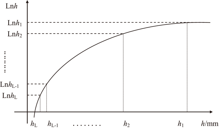
The thickness partitioned method is adopted by means of the natural logarithm as shown by Fig. 3, thickness of rolling pierce is defined as 2h in the X direction, and the logarithmic value of thickness is defined in the Y direction, since considering up and down surface as symmetric cooling process, half thickness h is used as subject for study. Logarithmic value of thickness is equidistantly divided into L-1 sections, the nodes number of which equal to L. Then exponential function of the nodes on the vertical coordinate can be separately calculated to obtain the value of the thickness h_i of each node. In the precondition of logarithmic value equidistance of thickness, the distance of two neighboring nodes on X-axis become larger as thickness increasing.

Fig. 3.

Diagram of thickness segment.

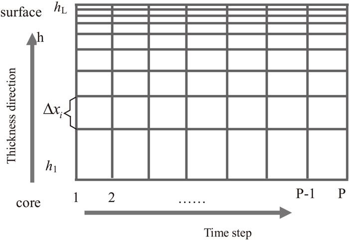
Diagram of thickness grid division of finite difference scheme is shown as Fig. 4.

Fig. 4.

Diagram of thickness grid division of finite difference scheme.

The heat conduction equation is used to solve the thermal radiation and convection heat transfer process.   

$$\frac{\partial T}{\partial t}=\alpha \frac{{\partial }^{2}T}{\partial x^2}$$(1)

Where α thermal diffusivity; t is heat exchange time, s.

To Solve the equation, the one dimensional implicit finite difference equation can be used as following   

$$\begin{array}{l}\frac{\alpha \cdot \mathrm{\Delta }t}{{(\mathrm{\Delta }{x}_i\cdot \mathrm{\Delta }{x}_{i-1})}^2}\cdot (-{(\mathrm{\Delta }{x}_{i-1})}^2\cdot T_{i+1}^p+\left[{(\mathrm{\Delta }{x}_i)}^2+{(\mathrm{\Delta }{x}_{i-1})}^2\right]\cdot \\ T_i^p-{(\mathrm{\Delta }{x}_i)}^2\cdot T_{i-1}^p)+T_i^p=T_i^{p-1}\end{array}$$(2)

Then,   

$$\begin{array}{l}{F}_i\cdot \left({(\mathrm{\Delta }{x}_{i-1})}^2\cdot T_{i+1}^p-\left[{(\mathrm{\Delta }{x}_i)}^2+{(\mathrm{\Delta }{x}_{i-1})}^2\right]\cdot T_i^p+{(\mathrm{\Delta }{x}_i)}^2\cdot T_{i-1}^p\right)\\ -T_i^p+T_i^{p-1}=0\end{array}$$(3)

Where,   

$$F_i=\frac{\alpha \cdot \mathrm{\Delta }t}{{(\mathrm{\Delta }{x}_i\cdot \mathrm{\Delta }{x}_{i-1})}^2}\cdot$$

The governing Eq. (3) is reduced to:   

$$\begin{array}{l}-{(\mathrm{\Delta }{x}_{i-1})}^2\cdot F_i\cdot T_{i+1}^p-\left[{(\mathrm{\Delta }{x}_i)}^2\cdot F_i+{(\mathrm{\Delta }{x}_{i-1})}^2\cdot F_i+1\right]\cdot \\ T_i^p-{(\mathrm{\Delta }{x}_i)}^2\cdot F_i\cdot T_{i-1}^p=T_i^{p-1}\end{array}$$(4)

Where, i=2, 3, …, L−1; p=1, 2, 3…, P.

According to the boundary conditions, the equations of boundary can be derived, finally a tridiagonal equation is obtained, and the temperature of each node in the final moments can be got by solving simultaneous equations of each node. The matrix form of the implicit difference equation is:   

$${\displaystyle \begin{array}{l}{\left[\begin{array}{c}{T}_1\\ T_2\\ \begin{array}{c}⋮\\ T_{L-1}\end{array}\\ T_L\end{array}\right]}^{p-1}=\\ \left[\begin{array}{ccccc}1+2\cdot {(\mathrm{\Delta }{x}_1)}^2\cdot F_1& -2\cdot {(\mathrm{\Delta }{x}_1)}^2\cdot F_1& & & \\ -{(\mathrm{\Delta }{x}_1)}^2\cdot F_2& \begin{array}{l}1+{(\mathrm{\Delta }{x}_2)}^2\cdot F_2\\ +{(\mathrm{\Delta }{x}_1)}^2\cdot F_2\end{array}& -{(\mathrm{\Delta }{x}_2)}^2\cdot F_2& & \\ & \ddots & \ddots & \ddots & \\ & & -{(\mathrm{\Delta }{x}_{L-2})}^2\cdot F_{L-1}& \begin{array}{l}1+{(\mathrm{\Delta }{x}_{L-1})}^2\cdot F_{L-1}\\ +{(\mathrm{\Delta }{x}_{L-2})}^2\cdot F_{L-1}\end{array}& -{(\mathrm{\Delta }{x}_{L-1})}^2\cdot F_{L-1}\\ & & & -2\cdot {(\mathrm{\Delta }{x}_L)}^2\cdot F_L& \begin{array}{l}1+{(\mathrm{\Delta }{x}_L)}^2\cdot F_L\\ +\cdot {(\mathrm{\Delta }{x}_L)}^2\cdot F_L\cdot B_L\end{array}\end{array}\right]\\ {\left[\begin{array}{c}{T}_1\\ T_2\\ \begin{array}{c}⋮\\ T_{L-1}\end{array}\\ T_L\end{array}\right]}^p+\left[\begin{array}{c}0\\ 0\\ \begin{array}{l}⋮\\ 0\end{array}\\ -2F_L\cdot B_L\cdot T_{\text{air}}\end{array}\right]\end{array}}$$(5)

Where, Biot numeral is $B_L=\frac{h_{\text{u}}\mathrm{\Delta }{x}_L}{\lambda }$; Fourier number is $F_i=\frac{\lambda \cdot \mathrm{\Delta }t}{c_{\text{p}}\cdot \rho \cdot {(\mathrm{\Delta }{x}_i)}^2}$; λ is thermal conductivity, W/(mK); c_p is Constant pressure heat capacity, J/(kgK); ρ is density of steel, kg/m³; h_u is Heat transfer coefficient.

To solve the tridiagonal equations, Thomas algorithm is used and the concrete solving steps are shown as following.

(1) Setting T_i = P_iT_i+1 + Q_i, then $P_1=\frac{2\cdot {(\mathrm{\Delta }{x}_1)}^2\cdot F_1}{1+2\cdot {(\mathrm{\Delta }{x}_1)}^2\cdot F_1}$, $Q_1=\frac{T_1{}^{p-1}}{1+2\cdot {(\mathrm{\Delta }{x}_1)}^2\cdot F_1}$;

(2) If i=2, 3, …, L−1, L, then $P_i=\frac{{(\mathrm{\Delta }{x}_i)}^2\cdot F_i}{1+{(\mathrm{\Delta }{x}_i)}^2\cdot F_i+{(\mathrm{\Delta }{x}_{i-1})}^2\cdot F_i},$, $Q_i=\frac{T_i{}^{p-1}+{(\mathrm{\Delta }{x}_{i-1})}^2\cdot F_i\cdot T_{i-1}}{1+{(\mathrm{\Delta }{x}_i)}^2\cdot F_i+{(\mathrm{\Delta }{x}_{i-1})}^2\cdot F_i}$;

(3) T_L^p = Q_L;

(4) If i= L, L−1, …, 2, 1, then T_L−1^p, T_L−2^p, …, T₂^p, T₁^p can been calculated in turn.

4. Calculation of Heat Transfer Coefficient

4.1. Heat Transfer of Thermal Radiation Process

Thermal radiation heat flux of steel plate surface q_u and heat transfer coefficient h_u are   

$$q_{\text{u}}=\epsilon \cdot \sigma \cdot \left[{\left(\frac{T_{\text{s}}+273}{100}\right)}^4-{\left(\frac{T_{\text{air}}+273}{100}\right)}^4\right]$$(6)

  

$$h_{\text{u}}=\frac{q_{\text{u}}}{T_{\text{s}}-T_{\text{air}}}$$(7)

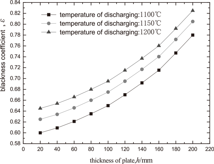
Where σ is thermal constant; T_s is temperature of plate surface, °C; T_air is air temperature, °C. ε is blackness coefficient of steel plate,¹⁶⁾ it is a function of thickness h and temperature T in °C such that:   

$$\epsilon =\frac{T}{1\mathrm{\hspace{0.17em} }000}\cdot \frac{h}{1\mathrm{\hspace{0.17em} }000}\left(\frac{3.74\times h}{1\mathrm{\hspace{0.17em} }000}+0.16\right)+\text{0}\text{.602}$$(8)

Relation of blackness coefficient and plate thickness is shown by Fig. 5.

Fig. 5.

Relation diagram of steel thickness and blackening coefficient.

Oxide scale thickness will increase during the process of heating in furnace, transporting in roll table as well as rolling in plate mill, and it will influence the heat transfer process of the steel plate, so it is meaningful to study the changing process of oxide scale thickness, diagram of oxide scale thickness as time changing is shown by Fig. 6.

Fig. 6.

Diagram of oxide scale thickness as time changing.

Calculating model of Oxide scale thickness is   

$$H_{\text{sn}}=K.\sqrt{{\left(\frac{H_{\text{so}}}{K}\right)}^2+\mathrm{\Delta }t}$$(9)

  

$$K={10.0}^{k_1\times {log}_{10}^{T_{\text{s}}}+k_2}$$(10)

Where T_s is temperature of plate surface, °C; k₁, k₂ growth coefficient of oxide scale; H_so is initial oxide thickness of plate, mm; H_sn is new oxide scale thickness of plate, mm; Δt is growth time of oxide scale, s;

Oxide scale has great effect on heat conduction between water and steel plate in fast cooling process, heat transfer coefficient will decrease as thickness of oxide scale increasing, and correction factor can be defined as k_s to quantify effect on the heat transfer coefficient by thickness of oxide scale.   

$$k_{\text{s}}=\frac{T_s-\frac{\lambda \cdot H_{\text{sn}}.(T_{\mathrm{\Delta }hs}-T_{\text{s}})}{{\lambda }_{\text{s}}.\mathrm{\Delta }{h}_s}-T_{\infty }}{T_s-T_{\infty }}$$(11)

Where λ_s is thermal conductivity of oxide scale, W/m°C; T_s is temperature of plate surface, °C; λ thermal conductivity of steel plate, W/m°C; T_∞ temperate of water, °C; Δh_s is distance to the surface of plate in thickness direction, mm; T_Δhs temperature difference from surface to Δh_s of plate, °C.

The convective heat transfer accounts for 7%–10% of thermal radiation heat transfer in ultra-heavy plate rolling process. The correct factors of the convective heat transfer of heat flux is   

$$k_{\text{h}}=\frac{e^{n^2}}{n^2}\cdot \left(1-\frac{2}{\sqrt{\pi }}{\int }_{\hspace{0.17em}0}^{\hspace{0.17em}n}{e}^{-z}dz\right)-\frac{1}{n^2}+\frac{2}{\sqrt{\pi }\times n}$$(12)

The final thermal radiation heat transfer coefficient is   

$$h_{\text{u}}=k_{\text{s}}\cdot k_{\text{h}}\cdot \frac{q_{\text{u}}}{T_{\text{s}}-T_{\text{air}}}$$(13)

4.2. The Heat Transfer of Water Cooling Process

Energy conservation is fundamental principles to solve the heat transfer coefficient in water cooling process, released heat quantity from steel plate equivalents to the one taken away by cooling water. To simplify the process, both surface of steel plate is considered as cooling uniformity, and then released heat quantity from steel plate is   

$$\mathrm{\Delta }E=C_p.m.dT=C_p\cdot \rho \cdot A\cdot h\cdot dT$$(14)

Where A is heat transfer surface area of plate, m²; h is plate thickness, m; dT is average temperature drop of plate, °C; C_p is specific heat of steel plate, kJ/kg. °C; ρ is density of steel, kg/m³.

Heat quantity taken away by cooling water is   

$$\mathrm{\Delta }Q=h_w\cdot \left(T-T_{\infty }\right)\cdot A\cdot d\tau$$(15)

Where dτ is heat transfer time, s; T_∞ temperate of water, °C; h_w is heat transfer coefficient of water cooling.

According to the law of conservation of energy, Heat quantity taken away by cooling water equals to the heat transfer in water cooling process.   

$$\mathrm{\Delta }E=\mathrm{\Delta }Q$$(16)

  

$$h_w\cdot \left(T-T_w\right)\cdot A\cdot d\tau =C_p\cdot \rho \cdot A\cdot h\cdot dT$$(17)

The heat transfer coefficient of water cooling is   

$$h_w=\frac{C_p\cdot \rho \cdot h\cdot dT}{\left(T-T_w\right)\cdot d\tau }$$(18)

  

$$dT=\frac{(T_s-T_w)\cdot f_s\cdot P_s}{h\cdot v\cdot C_p\cdot \rho }$$(19)

Where P_s is pressure of jet nozzle, MPa; f_s is water flow of jet nozzle, L/min; C_p is specific heat of steel plate, kJ/kg. °C; v is roll speed of plate, m/s; h is thickness of plate, mm.

4.3. The Heat Transfer of Rolling Process

In plate rolling process, horizontal surface contacts with the roll surface, according to relationship of thermal equilibrium, when temperatures drops by dT in a certain time equaling to dτ, which meets the following equation:   

$$c_p\rho v\text{d}t=h_{r}F(T_s-T_r)\text{d}\tau$$(20)

Where T_s temperate of steel plate, °C; T_r temperate of roller, °C; F is heat transfer surface area of plate and roller, m².

Then,   

$$h_r=\frac{c_p\rho v\text{d}T}{F(T_s-T_r)\text{d}\tau }$$(21)

The calculation formulas of contact temperature drop in rolling process is   

$$dT\text{=}\frac{4\beta \sqrt{\frac{{\kappa }_s\cdot \mathrm{\Delta }\tau }{\pi }}}{c_p\rho h}(T_s-T_r)$$(22)

Where β is efficiency of heat conduction of work piece and roller   

$$\beta =\frac{{\lambda }_r/\sqrt{{\kappa }_r}}{{\lambda }_s/\sqrt{{\kappa }_s}+{\lambda }_r/\sqrt{{\kappa }_r}}$$(23)

Where λ_r is thermal conductivity of roller, W/(mK); λ_s is thermal conductivity of steel plate, W/(mK); κ_r is thermal conductivity of roller; κ_s is thermal conductivity of steel plate.

5. Results and Discussion

The near surface heat transfer coefficient of the ordinary laminar flow cooling process is usually situated between 1000 and 2500 W/(m²∙°C), but the one of instant cooling is between 3000 to 5000 W/(m²∙°C), so in the study of the effect of heat transfer coefficient on the temperature field of steel plate, heat transfer coefficient can be selected as 2000 W/(m²∙°C), 3000 W/(m²∙°C), 4000 W/(m²∙°C) and 5000 W/(m²∙°C). The initial temperature 1150°C, the cooling time is 10 s, the thickness of the steel plate is 300 mm, and the variation of the near surface temperature changed over time with the different heat transfer coefficient is shown in Fig. 7.

Fig. 7.

Temperature distributed regularity with different heat transfer coefficients.

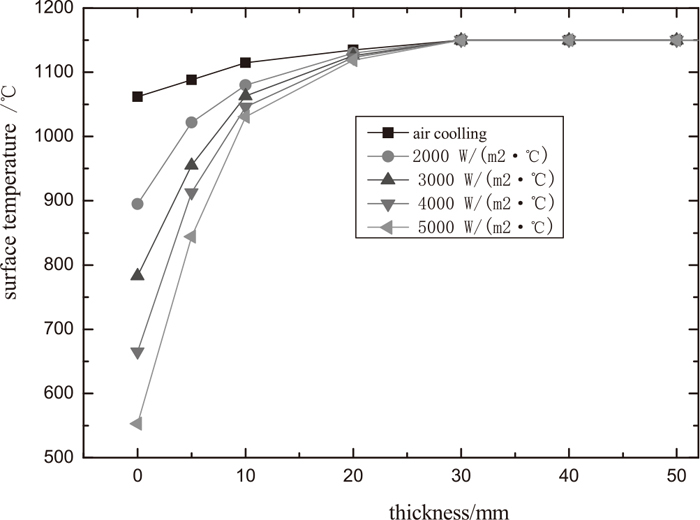
Figure 7 shows that temperature difference between near surface and center increases as the heat transfer coefficient increasing, when heat transfer coefficient changes from 2000 W/(m²∙°C) to 5000 W/(m²∙°C), corresponding temperature difference between near surface and center increases from 247°C to 603°C. The temperature at the position of a quarter of the thickness as well as that in the center of the steel plate tends to be consistent.

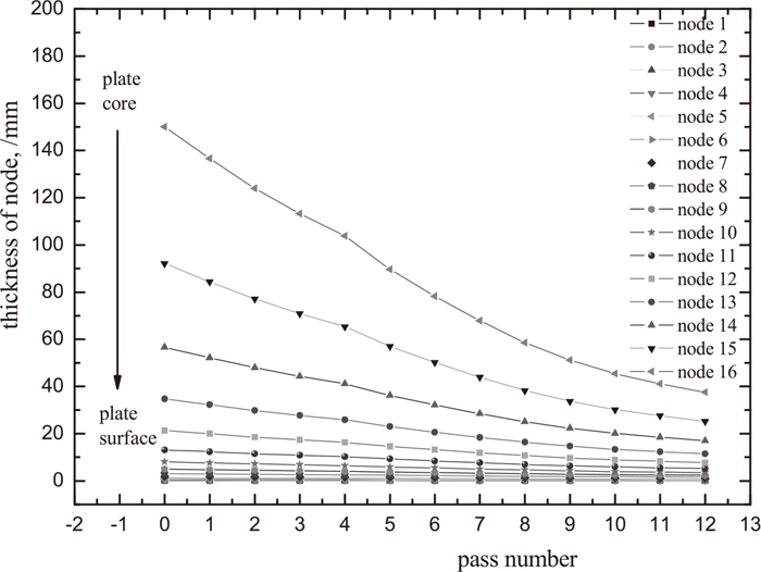
The thickness partitioned method is based on principle of equal distance between each thickness logarithm value as shown in Fig. 3 above. The rolling schedule is calculated with 12 passes, Thickness and its Logarithm value distribution of each node with half thickness is shown by Table 2 and Fig. 8.

Table 2. Thickness and its Logarithm value distribution of each node.

Fig. 8.

Thickness distribution of each node with increasing of pass number.

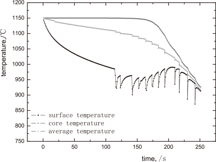
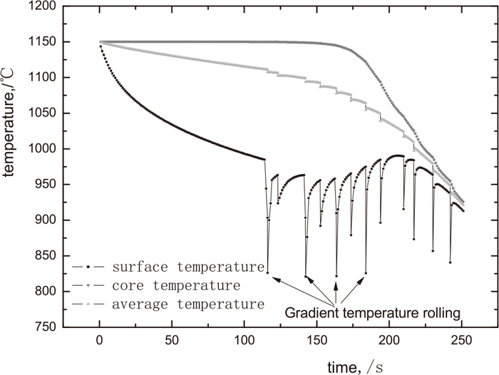
The temperature distributions for the traditional uniform temperature rolling process and the gradient temperature rolling are presented in Figs. 9 and 10. Instant cooling processes are carried out before pass1, pass3, pass 5 and pass 7, the surface temperature of those passes are decreased to about 820°C, which are obviously lower than traditional uniform temperature rolling processes.

Fig. 9.

The temperature distributions for traditional uniform temperature rolling process.

Fig. 10.

The temperature distributions of gradient temperature rolling process.

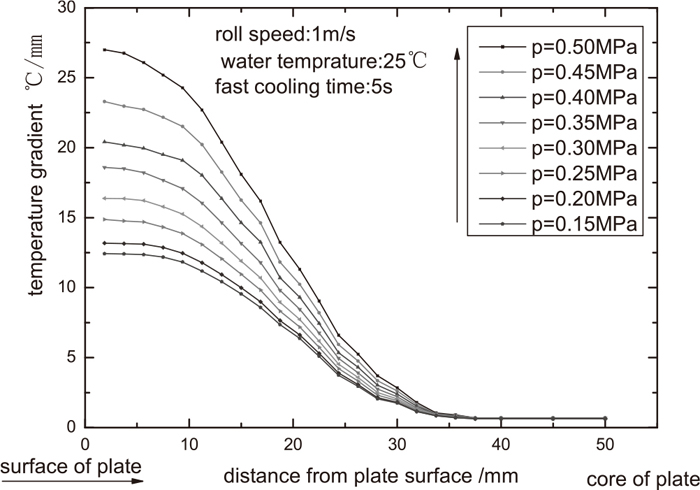
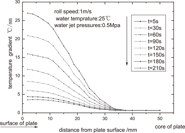
The temperature gradient distribution in thickness direction during fast cooling process with water jet pressure equaling to 0.5 MPa is shown in Fig. 11, maximum value near surface of plate can reach 27.4°C/mm, and temperature gradient decreases from near surface to a quarter of thickness and its decreasing range becomes smaller gradually as cooling time extending. The decreasing range of temperature gradient from a quarter of thickness to half thickness is less than that from the near surface to a quarter of thickness. The average temperature gradient near the center is around 1.5°C/mm, maximum temperatures difference of center and surface are about 573.4°C. The temperature gradient distribution in thickness direction with different water jet pressure is shown in Fig. 12, temperature gradient decreases as water jet pressure reducing. So, the lower is the water jet pressure, the worse is effect of temperature gradient rolling.

Fig. 11.

Temperature gradient change rules over time.

Fig. 12.

Temperature gradient change rules with different water jet pressures.

As described above, gradient temperature rolling changes plate temperature field distribution, even it improves the microstructure property of the plate center as well as the deformation uniformity in thickness direction, but it also increases the rolling load such as rolling force rolling torque and so on. Rolling schedule is calculated as shown in Table 3.

Table 3. Rolling schedule in gradient temperature rolling process.

pass number	Roll status	Entry Thickness, /mm	Exit Thickness, /mm	Rolling force reference, /kN	Rolling torque reference, /kN.m	Surface temperature, /°C	Core temperature, /°C	Average temperature, /°C
1	GTR	300	273.2	29509.68	3264.3	826.3	1149.7	1107.4
2		273.2	247.83	27184.32	2918.63	923.8	1149.6	1102.7
3	GTR	247.83	226.42	29184.72	3333.33	821.1	1148.7	1094
4		226.42	207.69	26318.52	3246.1	892.1	1147.7	1086.6
5	GTR	207.69	179.34	28920.48	3395.86	821.5	1144.7	1077.5
6		179.34	156.43	28677.96	3272.88	879.2	1137.8	1067.4
7	GTR	156.43	135.75	29215.68	3598.01	825.9	1121.8	1054.7
8		135.75	117.23	34148.88	3283.54	896.6	1093.7	1039
9		117.23	102.43	32609.4	2977.91	915.5	1045.2	1017.1
10		102.43	90.93	31220.4	2085.72	873.5	1025.1	997.5
11		90.93	82.34	29497.08	1907.542	857	988	967.4
12		82.34	75.00	279933.7	1646.515	840.9	954.7	936.1

Table 3 shows that gradient temperature rolling mode is used in pass 1, pass 3, pass 5 and pass 7, calculated rolling force reference and rolling torque reference are slightly larger than neighboring values by about 10%. This indicates that Gradient temperature rolling process is really not affected rolling load too much. Radiant pyrometers are installed in upstream and downstream of stand, surface temperature of plate can be measured at any moment while rolling is in progress. Therefore, measured temperature can be used to verify the calculation temperature. In order to obtain clear contrast effect, node number is selected as 16, 12, 8 and 4 with half thickness, and then, comparison of measured temperature and calculated temperature can be obtained with different partitioned node number as shown by Fig. 13.

Fig. 13.

comparison of measured and calculated temperature with different partitioned node number.

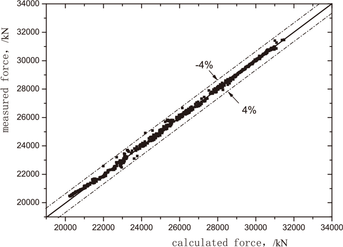
Figure 13 shows that the more is the node number, the more accurate is the temperature prediction precision. As node number increasing, prediction difference with the actually measured data becomes smaller, when node number equals to 16, prediction difference can be controlled with ±5°C. High precision of temperature prediction can provide the prediction precision of rolling force, especially rolling with the gradient temperature rolling passes. Deviation of calculated force and measured force can be controlled with ± 4.0% as shown by Fig. 14.

Fig. 14.

Deviation of calculated force and measured force.

6. Conclusions

(1) Temperature control technology by finite difference scheme with thickness unequally partitioned method is investigated in gradient temperature rolling. Partition method is adopted by means of equidistance logarithmic value for thickness and gets the effect of more detailed grid on surface and rough grid in the core.

(2) The industrial testing result illustrates that calculated rolling force reference and rolling torque reference are slightly larger than neighboring values by about 10% when gradient temperature rolling mode is used in pass 1, pass 3, pass 5 and pass 7.

(3) From comparison of measured temperature and calculated temperature, it indicates that prediction difference can be controlled with ±5°C when node number equals to 16 with half thickness and deviation of calculated force and measured force can be controlled with ± 4.0%.

Acknowledgements

The authors wish to acknowledge the financial support received from State Key Laboratory of Rolling and Automation, Northeastern University, China, under the National Natural Science Foundation of China (GrantNo. 51504061) and the Fundamental Research Funds for the Central Universities (No. 100307004).

References

• 1)   Y.  Hou,  Y. J.  Tao and  X. L.  Huai: Appl. Therm. Eng., 62 (2014), 613.
• 2)   W.  Deng,  D. W.  Zhao and  X. M.  Qin: Comput. Mater. Sci., 47 (2009), 439.
• 3)   S.  Dobatkin,  J.  Zrnik and  I.  Mamuzi: Metalurgija, 48 (2009), 157.
• 4)   H.  Dong and  X. J.  Sun: Curr. Opin. Solid State Mater. Sci., 9 (2005), 269.
• 5)   Y. Y.  Fu,  P.  Yang,  W. Y.  Yang and  X. Q.  Sun: J. Univ. Sci. Technol. Beijing, 22 (2006), 170.
• 6)   H.  Han,  J.  Lee,  H.  Kim and  Y.  Jin: J. Mater. Process. Technol., 128 (2002), 216.
• 7)   S.  Serajzadeh and  T. A.  Karimi: Int. J. Model. Simul., 24 (2004), 42.
• 8)   E.  Liu,  D.  Zhang,  J.  Sun,  L.  Peng,  B.  Gao and  L.  Su: J. Iron Steel Res. Int., 19 (2012), 39.
• 9)   W.  Yu,  G. S.  Li and  Q. W.  Cai: J. Mater. Process. Technol., 217 (2015), 317.
• 10)   T.  Zhang,  B. X.  Wang,  Z. D.  Wang and  G. D.  Wang: ISIJ Int., 56 (2016), 179.
• 11)   T. L.  Fu,  Z. D.  Wang,  Y.  Li,  J. D.  Li and  G. D.  Wang: Appl. Therm. Eng., 70 (2014), 800.
• 12)   M.  Visaria and  I.  Mudawar: J. Electron. Packag., 129 (2007), 452.
• 13)   S. C.  Chapra and  R. P.  Canale: Numerical Methods for Engineers, McGraw-Hill, New York, (1998), 832.
• 14)   J. L.  Marcelin: Int. J. Adv. Manuf. Technol., 32 (2007), 711.
• 15)   M.  Islam,  S. H.  Mallik and  M.  Kanoria: Appl. Math. Mech., 32 (2011), 1315.
• 16)   H.  Wang,  W.  Yu and  Q. W.  Cai: J. Mater. Process. Technol., 212 (2012), 1825.