Computational Simulation Model for Metallurgical Effects during EAF Refining Stage: Waiting and Arcing Time

Abstract

3D computational fluid dynamics models using Fluent were developed to investigate the steel melt flow during waiting and arcing time. Both models were transient that analyzed 60 seconds to investigate the flow characteristics considering variation in steel melt thermo-physical parameters and operating conditions. The velocity of melt movement was high enough to make a turbulent flow (solved with realize k-ε turbulence model).

It was found that the steel melt flow velocity increases by a combined effect of the steel melt temperature and composition, and slag pressure. The slag pressure increases by a double effect of slag density and height, and the steel melt fluid flow velocity changes with the slag pressure. The effect of the slag thickness is more significant than the effect of thermo-physical properties of steel melt. Although, the maximum steel melt velocity “during arcing time” may be as large as 0.67 m/s located at steel met outlet, the melt exhibits completely dead zones with minimum flow velocity distribution especially at the bottom and circumference areas. This indicates the importance of combined stirring and large reaction rates to achieve a complete homogeneous melt especially at bottom and circumference areas.

1. Introduction

The refining process is the controlled process required to produce different grades with different steel melt compositions according to the desired steel grade to be produced. It is achieved through continuous arcing by the three graphite electrodes combined with continuous oxidation using sidewall oxygen injection. As a result, the melt fluidity increases as a result of increasing the steel melt temperature, decreasing carbon content, and increasing slag thickness, density and pressure.

During the refining stage arcing time, there is steel melt heating via three graphite electrodes located at the furnace center. It can be represented by the forced convection. In forced convection, the flow is induced by external source. This effect occurs as a result of continuous arcing by the three graphite electrodes, combined with continuous oxidation from the side wall oxygen injection. This change in temperature and composition results in changes in the melt temperature, composition and slag thickness. This results in change in the steel melt fluidity.

During the last 20 years, many researches were done to investigate the steel melt flow. The study done by Wang et al.^1,2) indicated that convection and radiation heat transfer mechanisms are responsible for heating and melting iron scrap in the steelmaking process. Kazak et al.^3,4,5,6) concluded that the Lorenz force had the major effect on the origination of the vortex motion of a melt in bottom electrode direct current (DC) EAF.

Teng et al.⁷⁾ investigated the effect of ArcSave method on the enhancement of scrap and ferrochromium melting and the reduction of energy consumption with homogeneous bath temperature. Alexis et al.⁸⁾ predicted the temperature measurements and the combined effect of heating and induction stirring during ladle treatment using a 3D simulation model. Karalis et al.⁹⁾ developed a 3D mathematical model, to compute the electric potential, electric current density and Joule heat distributions during ferronickel smelting process in EAF. Smirnov et al.^10,11) developed a numerical simulation of electromagnetic stirring of metal melt in a direct current (DC) arc furnace to calculate the turbulence using the large eddy simulation (LES) method. Wang et al.¹²⁾ developed a 3D model to predict the electromagnetic stirring effect of the molten bath as current, temperature field distribution in the EAF for the MgO production using FLUENT.

Nazari¹³⁾ developed a 3D linear electrical model for the AC arcs for estimation of the thermal radiation received by different parts of the furnace. Sanchez et al.¹⁴⁾ developed a radiation model for predicting hot spots formation for an industrial EAF with long arc operation of 45 cm. Yigit et al.¹⁵⁾ developed a 3D CFD model predicting temperature distributions of the inclusion of combustion reactions and radiation interactions inside the EAF.

Chun et al.¹⁶⁾ showed that the combined stirring of gas blowing and induction stirring was effective for both bulk mixing and the removal of inclusions in the ASEA-SKF ladle using 3D numerical model. Liu et al.¹⁷⁾ showed that increasing flow rate and improving stirring, affected the molten bath in eccentric bottom tapping (EBT) region, and would decrease mixing time and improve stirring ability. Peranandhanthan et al.¹⁸⁾ measured the slag eye area in an axi-symmetrical water model of an argon stirred ladle using video, the results showed that the slag eye area increased as the gas flow rate and depth of bulk liquid increased. Geng et al.¹⁹⁾ predicted the collision and aggregation among inclusions in the ladle with different porous plug configurations, the results showed that the porous plug configuration had a major effect on the inclusion removal process in ladle. Liu et al.²⁰⁾ showed that the flow pattern of the molten steel in a three-phase argon gas-stirred ladle was dependent on the plug configurations and argon gas flow rate. Wei et al.²¹⁾ developed a water model experiment and a computational fluid dynamic model in the EAF molten bath, the results showed that the interaction among the bottom-blowing gas streams could accelerate the fluid flow and decrease the volume of the dead zone.

Some researchers^22,23,24) have reported the effect of foam slag and injected gas on the decarburization and melt flow in Electric Arc Furnace. However, others^25,26,27) investigated the bottom gas stirring using numerical and physical models. In particular, Kumar²⁸⁾ predicted the onset of droplet formation, and the critical gas flow rate required for droplet.

The interaction between the arc and the molten bath was investigated by some researchers.^29,30,31) In particular Gonzalez et al.³²⁾ developed a radiation model predicting hot spots formation for an industrial Electric Arc Furnace with long arc operation of 45 cm. Ramírez et al.³³⁾ found that in the absence of gas injection, the electromagnetic body forces dominate the fluid flow in the bath region.

All these studies showed that no single model can include all parameters during the refining stage, as the refining stage includes in addition to dynamic flow conditions, some other conditions resulting from chemical reactions and temperature changes. It is also shown that there is no comparative analysis of the effect of slag thickness and thermo-physical properties of steel during refining stage waiting and arcing time.

The aim of this work is to investigate the effect of actual refining stage conditions “actual thermo-physical parameters and operating conditions” during waiting and arcing time. The operating conditions are presented by the slag thickness and the thermo-physical properties of steel. The slag thickness varies from 0.05–0.30 m. The thermo-physical properties of the steel also vary within the effective range of temperature 1550–1700°C and carbon content 0.02–0.20% C. The thermo-physical properties of the melt include temperature dependent properties, namely; density, viscosity, heat capacity and thermal conductivity. Moreover, the change of steel melt composition affects the slag composition and density. These properties affect the steel melt velocity distribution. In the current work, the melt flow velocity distribution is investigated at different refining conditions during the waiting and arcing time. During the waiting time, there is neither arcing nor oxygen injection and it can be represented by natural convection. In natural convection, the flow is induced by the differences between fluid densities which result due to temperature changes, it occurs due to temperature differences which affect the density, and thus relative buoyancy, of the fluid. However, forced convection uses externally induced flow resulting in fluid movement and increased rate of heat exchange. It represented by a three graphite electrodes each 600 mm diameter with arcing power of 120 MW. The rates of heat transfer using forced convection are higher than that for natural convection, where, the higher the fluid velocities, the higher the rate of heat transfer. The refining conditions include different slag thickness combined with different steel melt temperature and chemistry. This study is based on previous study done by Elkoumy et al.³⁴⁾ for simulation of EAF refining stage.

2. Materials and Methods

2.1. Computational Model

The developed CFD model aims to simulate the steel melt velocity in an industrial EAF of 225-ton capacity during EAF refining stage arcing time. The model investigates the effect of different low carbon steel grades in the range 0.02–0.20%C, and melt temperature range 1550–1700°C during arcing time. Furthermore, it investigates the effect of different operating parameters “mainly slag density, thickness (0.05–0.30 m) and pressure” during waiting and arcing time.

The CFD model aims to simulate the actual refining conditions in industrial EAF of 225-ton capacity during arcing time using forced convection phenomena. These conditions include the actual metallurgical and operation variables. Different mesh sizes were tested, while the used mesh size consists of 550000 elements. The used governing equations are continuity, momentum conservation equations and equations for the turbulence model (Realize k-ε) are used based on previous studies.^{35,36,37,38,39)}

2.1.1. Governing Equations

2.1.1.1. Continuity Equations:

For Non-steady state, Incompressible flow ρ = const; $\frac{\partial \rho }{\partial t}=0$   

$$\frac{\partial U}{\partial x}+\frac{\partial V}{\partial y}+\frac{\partial W}{\partial z}=0$$

2.1.1.2. Momentum Equations:

Momentum Equation “Navier Stokes Equation” X-Direction:   

$$\begin{array}{l}\frac{\partial U}{\partial t}+U\frac{\partial U}{\partial x}+V\frac{\partial U}{\partial y}+W\frac{\partial U}{\partial z}=-\frac{1}{\rho }\frac{\partial P}{\partial x}+\frac{\partial }{\partial x}\left(2\mathrm{\hspace{0.17em} }{\mu }_{\mathrm{e}}\frac{\partial U}{\partial x}\right)\\ +\frac{\partial }{\partial y}(2\mathrm{\hspace{0.17em} }{\mu }_{\mathrm{e}}\left(\frac{\partial U}{\partial y}+\frac{\partial V}{\partial x}\right)+\frac{\partial }{\partial z}(2\mathrm{\hspace{0.17em} }{\mu }_{\mathrm{e}}\left(\frac{\partial U}{\partial z}+\frac{\partial W}{\partial x}\right)\end{array}$$

Momentum Equation “Navier Stokes Equation” Y-Direction:   

$$\begin{array}{l}\frac{\partial V}{\partial t}+ U\frac{\partial V}{\partial x}+V\frac{\partial V}{\partial y}+W\frac{\partial V}{\partial z}=-\frac{1}{\rho }\frac{\partial P}{\partial y}+ \frac{\partial }{\partial y}\left(2\mathrm{\hspace{0.17em} }{\mu }_{\mathrm{e}}\frac{\partial V}{\partial y}\right)\\ + \frac{\partial }{\partial x}(2\mathrm{\hspace{0.17em} }{\mu }_{\mathrm{e}}\left(\frac{\partial V}{\partial x}+\frac{\partial U}{\partial y}\right)+ \frac{\partial }{\partial z}(2\mathrm{\hspace{0.17em} }{\mu }_{\mathrm{e}}\left(\frac{\partial V}{\partial z}+\frac{\partial W}{\partial y}\right)+\mathrm{g}\end{array}$$

Momentum Equation “Navier Stokes Equation” Z-Direction:   

$$\begin{array}{l}\frac{\partial W}{\partial t}+U\frac{\partial W}{\partial x}+V\frac{\partial W}{\partial y}+W\frac{\partial W}{\partial z}=-\frac{1}{\rho }\frac{\partial P}{\partial Z}+\frac{\partial }{\partial Z}\left(2\mathrm{\hspace{0.17em} }{\mu }_{\mathrm{e}}\frac{\partial w}{\partial Z}\right)\\ + \frac{\partial }{\partial x}(2\mathrm{\hspace{0.17em} }{\mu }_{\mathrm{e}}\left(\frac{\partial W}{\partial x}+\frac{\partial U}{\partial z}\right)+\frac{\partial }{\partial y}(2\mathrm{\hspace{0.17em} }{\mu }_{\mathrm{e}}\left(\frac{\partial W}{\partial z}+\frac{\partial V}{\partial y}\right)\end{array}$$

2.1.1.3. Energy Equation

The Turbulent Kinetic Energy   

$$\frac{\partial k}{\partial t}+U\frac{\partial k}{\partial x}+V\frac{\partial k}{\partial y}+W\frac{\partial k}{\partial z}=\frac{\partial }{\partial x}\left[\frac{{\mu }_{\text{t}}}{{\sigma }_k}\frac{\partial k}{\partial x}\left]+\frac{\partial }{\partial y}\right[\frac{{\mu }_{\text{t}}}{{\sigma }_k}\frac{\partial k}{\partial x}\right]-\epsilon +\frac{G}{\rho }$$

  

$${\mu }_t=\rho C_{\mu }\frac{k^2}{\epsilon }$$

  

$$C_{\mu }=\frac{1}{A_0+A_S\frac{k{U}^{*}}{\epsilon }}$$

The Dissapation Kinetic Energy   

$$\begin{array}{l}\frac{\partial \epsilon }{\partial t}+U\frac{\partial \epsilon }{\partial x}+V\frac{\partial \epsilon }{\partial y}+W\frac{\partial \epsilon }{\partial z}=\frac{\partial }{\partial x}\left[\frac{{\mu }_{\text{t}}}{{\sigma }_{\epsilon }}\frac{\partial \epsilon }{\partial x}\right]+\frac{\partial }{\partial y}\left(\frac{{\mu }_{\text{t}}}{{\sigma }_{\epsilon }}\frac{\partial \epsilon }{\partial y}\right)\\ +\frac{\partial }{\partial k}\left[\frac{{\mu }_{\text{t}}}{{\sigma }_{\epsilon }}\frac{\partial \epsilon }{\partial z}\right]-\frac{C_2{\epsilon }^2}{k}+\frac{G}{\rho k}(C_{1}G-C_2)\end{array}$$

The arc power is presented in the energy equation as source term G³²⁾ is presented as follows:   

$$\begin{array}{l}G={\mu }_{eff}\{2\left[{\left(\frac{\partial {\upsilon }_x}{\partial x}\right)}^2+{\left(\frac{\partial {\upsilon }_y}{\partial x}\right)}^2+{\left(\frac{\partial {\upsilon }_z}{\partial x}\right)}^2\right]\\ +{\left(\frac{\partial {\upsilon }_y}{\partial x}+\frac{\partial {\upsilon }_x}{\partial y}\right)}^2 +{\left(\frac{\partial {\upsilon }_z}{\partial y}+\frac{\partial {\upsilon }_y}{\partial z}\right)}^2+{\left(\frac{\partial {\upsilon }_x}{\partial z}+\frac{\partial {\upsilon }_z}{\partial x}\right)}^2\}\end{array}$$

2.1.2. Assumptions

The following assumptions have been made while developing this computational model:

 1. Full coupling between governing equations.

 2. The waiting time was presented by natural convection.

 3. The arcing time was presented by forced convection.

 4. Driving forces are limited to buoyancy forces “for natural convection”.

 5. Driving forces are 120 MW arc power “for forced convection”.

 6. Liquid steel thermo-physical properties are varied within the temperature range 1823–1973 K and carbon range 0.02–0.20% C.

 7. The steel thermal properties (ρ, μ, k and Cp) are temperature dependent.

 8. The steel has variable viscosity and density at each temperature and carbon content.

 9. Physical characteristics of the medium are assumed to be uniform.

10. Walls remain at a constant temperature.

11. A fixed flat bath surface.

12. No slip condition between slag and steel surface, neither at all walls.

13. Slag layer influence is considered as a uniform load pressure.

14. Chemical reactions are neglected, but their effect appears on the slag thickness and density because the resulted FeO formation is taken into account. This is described later in detail.

15. No phase transformation; neither: solidification, melting, vaporization, condensation, or sub-limitation.

16. Heat losses from the top surface are neglected.

2.2. Operating Conditions

The actual operating conditions at EZZ Steel Company-Ain Sukhna Suez Egypt were used to provide data necessary for the computational model, for eccentric bottom tapping (EBT) EAF with 225-ton capacity under forced conditions. These data present the major affecting parameters during waiting and arcing time in this study, which are the variable slag thickness “0.05–0.30 m”, the melt temperature in the range 1550–1700°C and the composition in the range 0.02–0.20% C. This data was used to predict the thermo-physical properties of the steel.

The geometric modeling was transferred to FLUENT software as IGS file. The EAF drawing is illustrated in Figs. 1-a³⁴⁾ and 1-b. The parameters used to build the melt geometry are summarized in Table 1. The used composition range for the steel melt is listed in Table 2. The used composition range for the slag is listed in Table 3. The unit of %C, %Si, %Mn, % P, % S, % Cu, % Cr, % Ni, % Mo, % SiO₂, % CaO, % Al₂O₃, % Fe_xO_y, %FeO and Fe₂O₃ are in mass%. The thermo-physical properties of the steel melt and slag are illustrated in Table 4.^{41,42,43,44,45,46)} The slag weight is illustrated in Table 5, to illustrate the effect of slag thickness and density on slag weight above the steel melt. As assumed above stated as No.14, the formation of FeO in the slag phase is resulted from decarburization leading to an increase of slag thickness and weight as understood in Table 5, where the data were taken empirically at EZZ Steel. The slag pressure is illustrated in Table 6. The slag pressure is the input parameter, whose data are those taken at EZZ steel, and used for the simulation. The slag weight and pressure, can be calculated as per Eqs. (1), (2), where W_slag is the slag weight, ρ_slag is the slag density, is the slag cross section area, is the slag height, and is the slag cross section area. Furthermore, the slag pressure can be calculated as from the slag weight as shown in Eq. (3).   

$${\text{W}}_{slag}={\rho }_{slag}\times {\text{A}}_{slag}\times {\text{h}}_{slag}$$(1)

  

$${\text{P}}_{slag}={\rho }_{slag}\times {\text{A}}_{slag}\times \mathrm{9.81.}$$(2)

  

$${\text{P}}_{slag}=\frac{{\text{W}}_{slag}*9.81}{{\text{A}}_{slag}}.$$(3)

Fig. 1-a.

Detailed views of EAF.³⁴⁾

Fig. 1-b.

EAF top view from FLUENT.

Table 1. Plant Electric Arc Furnace melt geometry/dimensions.

Parameter	Molten Steel Volume	Large diameter	Melt height	Arc spot diameter	Length
Value	32	6.648	1.12	0.6	8.5
Unit	m3	M	m	m	m

Table 2. Steel melt chemical composition range “mass%”.

% C	% Si	% Mn	% P	% S	% Cr	% Ni	% Cu	% Mo
0.02–0.20	0.005–0.200	0.01–0.55	0.005–0.0500	0.02–0.05	0.03–0.23	0.02–0.12	0.04–0.060	0.01–0.04

Table 3. Typical slag composition range “mass%”.

% SiO2	% CaO	% Al2O3	% MgO	% FexOy	% FeO	% Fe2O3
16–23	32–46	4–5	7.8–9.6	16.84–43.35	14.4–38.5	1

Table 4. Thermo-physical properties of steel and slag.

Steel Temp; °C	Slag Temp; °C	% C	Steel Thermal Conductivity; W/(m K)	Steel Density; kg/m3	Steel Viscosity; kg/(s m)	Steel Specific Heat; J/(kg K)	Slag Density; kg/m3
1700	1750	0.020	34.99	6898	0.0039828	799.39	3152
1675	1725	0.035	34.99	6918	0.0041153	803.97	3078
1650	1700	0.050	34.99	6938	0.0042483	807.26	3040
1625	1675	0.075	34.99	6957	0.0043735	812.53	2983
1600	1650	0.100	34.99	6976	0.0044994	815.65	2949
1575	1625	0.150	34.99	6993	0.0046473	822.63	2926
1550	1600	0.200	34.99	7010	0.0047972	825.33	2864

Table 5. Variation in slag thickness (m) and weight (ton) at different temperatures and C %, for steel melt cross sectional area of 44.4 m².

Steel - slag characteristics					Slag weight “ton” as function of slag thickness “0.05–0.30 m”
Steel temperature; °C	Slag temperature; °C	% C	% FeO	Slag density; kg/m3	0.05	0.10	0.15	0.20	0.25	0.30
1700	1750	0.020	38.50	3151.6	7.0	14.0	21.0	28.0	35.0	42.0
1675	1725	0.035	32.65	3078.4	6.8	13.7	20.5	27.4	34.2	41.0
1650	1700	0.050	28.92	3040.1	6.8	13.5	20.3	27.0	33.8	40.5
1625	1675	0.075	24.69	2982.9	6.6	13.3	19.9	26.5	33.1	39.8
1600	1650	0.100	21.68	2948.7	6.6	13.1	19.7	26.2	32.8	39.3
1575	1625	0.150	17.44	2925.6	6.5	13.0	19.5	26.0	32.5	39.0
1550	1600	0.200	14.43	2864.3	6.4	12.7	19.1	25.5	31.8	38.2

Table 6. Variations in slag pressure (N/m²) for different temperatures and C% and slag thickness (m).

Steel - slag characteristics					Slag pressure “N/m2” as function of slag thickness “0.05–0.30 m”
Steel temperature; °C	Slag temperature; °C	% C	% FeO	Slag density; kg/m3	0.05	0.10	0.15	0.20	0.25	0.30
1700	1750	0.020	38.50	3151.6	1546	3092	4638	6183	7729	9275
1675	1725	0.035	32.65	3078.4	1510	3020	4530	6040	7550	9060
1650	1700	0.050	28.92	3040.1	1491	2982	4473	5965	7456	8947
1625	1675	0.075	24.69	2982.9	1463	2926	4389	5852	7315	8779
1600	1650	0.100	21.68	2948.7	1446	2893	4339	5785	7232	8678
1575	1625	0.150	17.44	2925.6	1435	2870	4305	5740	7175	8610
1550	1600	0.200	14.43	2864.3	1405	2810	4215	5620	7025	8430

At the end of the refining stage, the temperature and chemistry were measured during waiting and arcing time to investigate the effect of forced convection compared to natural convection on steel melt homogeneity.³⁴⁾

The temperature measurements made at the end of the refining stage before tapping “for natural convection condition” showed 1630–1650°C, and showed a variation only within a range from 28 to 92°C, at the receiving stage in the ladle refining furnace (LRF).³⁴⁾ The temperature measurements made at the end of the refining stage before tapping “for forced convection condition” showed 1630–1650°C and varied within a range of 66 to 74°C at the receiving stage in the LRF.³⁴⁾ The chemistry measurements made at the end of the refining stage before tapping “for natural convection condition” varied from 0.03–0.04% C, and varied from 0.0095 till 0.0117% C at the receiving stage in the LRF.³⁴⁾ Chemistry measurements made at the end of the refining stage before tapping “for forced convection condition” showed % C at 0.03–0.04% C and varying from 0.0003 to 0.0012% C at the receiving stage in the LRF.³⁴⁾

3. Model Verification

The developed model was verified by comparing the velocity distribution for forced convection at 60 sec with similar results provided by Arzpeyma³⁶⁾ as shown in Figs. 2, 3. Also, the velocity results obtained by the developed model were verified by analyzing the effect on the temperature and chemical measurements “mainly % C content” made at the end of the refining stage before tapping and the LRF arrival stage. These measurements were done for both which results in changes in natural and forced convection. The model validation results showed that the temperature and chemical composition measurements showed large variations between the EAF tapping stage at the end of the refining and the LRF arrival stage for natural convection, compared to forced convection. This indicates non-homogeneous temperature distribution, chemical distribution and transport characteristics in the steel melt for natural convection compared to forced convection. Moreover, the detailed model verification results are illustrated by Elkoumy et al.³⁴⁾

Fig. 2.

Steel melt velocity vector plot distribution reported by Arzpeyma.³⁸⁾

Fig. 3.

Steel melt velocity vector plot distribution reported by current study.

4. Results and Discussion

In the current research, CFD models are used to study the influence of slag thickness (varying from 0.05–0.30 m), thermo-physical properties of the molten steel at different carbon compositions (in the range 0.02–0.20% C) and temperature range 1550–1700°C of natural and forced convection; during refining stage inside the bath in an eccentric bottom tapping (EBT) EAF.

4.1. Waiting Time Natural Convection Computational Model

In natural convection mode, the flow driving force is generated from the temperature differences, which affect the density, and thus relative buoyancy, of the fluid.^{28,29,30,31,32,33,34)} The main steel melt flow parameter investigated is velocity distribution.

The fluid flow is simulated for natural convection without any energy source or bottom stirring to investigate the fluid flow characteristics at natural convection characteristics for 60 seconds. The results show that the maximum velocity distribution occurs at the steel melt outlet surface and at the longitudinal and transverse sections, as indicated from previous work done by Elkoumy et al.³⁴⁾ However, the minimum velocity distribution occurs at the bottom and the outer circumference.³⁴⁾ The results of the waiting time natural convection computational model are illustrated in Fig. 4 and Table 7.

Fig. 4.

Maximum steel melt velocity variation with different slag thickness, composition and temperature in natural convection.

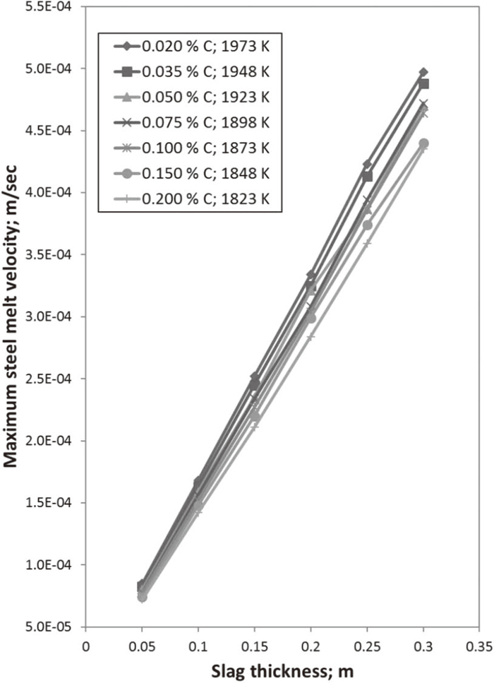
Table 7. Natural convection model results – maximum steel melt velocity “m/sec” with temperature “°C “ - % C – slag thickness “m”.

Operating Conditions			Maximum steel melt velocity; “m/s”
Steel Temperature; °C	% C	Convection Method	0.05	0.10	0.15	0.20	0.25	0.30
1700	0.020	Natural	8.49 e-05	1.68 e-04	2.52 e-04	3.34 e-04	4.23 e-04	4.97 e-04
1675	0.035	Natural	8.25 e-05	1.63 e-04	2.45 e-04	3.25 e-04	4.13 e-04	4.88 e-04
1650	0.050	Natural	8.03 e-05	1.59 e-04	2.35 e-04	3.21 e-04	3.87 e-04	4.70 e-04
1625	0.075	Natural	7.79 e-05	1.56 e-04	2.34 e-04	3.08 e-04	3.94 e-04	4.72 e-04
1600	0.100	Natural	7.73 e-05	1.52 e-04	2.27 e-04	3.04 e-04	3.86 e-04	4.64 e-04
1575	0.150	Natural	7.43 e-05	1.48 e-04	2.20 e-04	2.99 e-04	3.74 e-04	4.40 e-04
1550	0.200	Natural	7.22 e-05	1.42 e-04	2.11 e-04	2.84 e-04	3.59 e-04	4.35-04

4.1.1. Effect of Thermo-Physical Properties of Steel Melt on Velocity Distribution

The fluid flow was simulated for natural convection at varying temperature conditions during the refining stage. The aim of the simulation is to investigate the fluid flow characteristics at natural convection characteristics for 60 seconds with different thermo-physical properties at different steel melt temperatures and chemistry.

The effect of changes in steel melt thermo-physical properties on steel flow velocity is illustrated in Table 7 and Figs. 5, 6, 7. The maximum velocity distribution is exhibited at the steel melt outlet surface and at the longitudinal and transverse sections.³⁴⁾ The minimum velocity distribution exists at the bottom and outer circumference.³⁴⁾ Based on the results, it can be shown that the effect of steel melt thermo-physical properties on the steel melt flow velocities is found to be minor compared to slag thickness conditions effect (which will be shown in next section). This could be deduced by comparing the different conditions during the refining stage (temperature and composition) for the same slag thickness. The studied conditions were based on changing the density, viscosity, heat capacity and thermal conductivity, of the steel melt during the refining stage, without altering the slag thickness.

Fig. 5.

Velocity vector distribution for natural convection at 60 sec at 0.20% C, 1823 K and 0.15 m slag thickness.

Fig. 6.

Vector velocity distribution for natural convection at 60 sec at 0.02% C, 1973 K and 0.15 m Slag Thickness.

Fig. 7.

Maximum steel melt velocity variation with different steel melt temperature and composition in 60 Sec natural convection at 0.15 m slag thickness.

The effect of the thermo-physical on steel melt flow can be explained by comparing the steel melt velocity at constant slag thickness of 0.15 m for 0.20% C and 1823 K compared with 0.02% C and 1973 K, as shown in Figs. 5, 6, 7. The maximum velocity distribution is presented at steel melt outlet surface. The maximum steel melt velocity is 2.11 * 10⁻⁴ m/sec at 0.15 m slag thickness, 0.20% C, and 1823 K as shown in Fig. 5, compared with 2.52 * 10⁻⁴ m/sec at 0.15 m slag thickness, 0.02% C, and 1973 K as shown in Fig. 6.

The selected cases for comparison are at constant slag thickness of 0.15 m. The cases are”0.20% C, 1550°C”, “0.15% C, 1575°C”, “0.10% C, 1600°C”, “0.075% C, 1625°C”, “0.05% C, 1650°C”, “0.035% C, 1675°C” and “0.02% C, 1700°C”, “0.20% C, 1550°C”.

4.1.2. Effect of Slag Thickness on Velocity Distribution

The fluid flow was simulated for natural convection at different slag thickness conditions during the refining stage. The aim of the simulation is to investigate the fluid flow characteristics at natural convection characteristics for 60 seconds with different slag thickness.

The results of the effect of slag thickness on steel flow velocity are illustrated in Table 7 and Figs. 8, 9. The maximum velocity distribution is exhibited at the steel melt outlet surface and at the longitudinal and transverse sections. The minimum velocity distribution exists at the bottom and outer circumference. Based on the results, it can be shown that the effect of slag thickness on the steel melt flow velocities is found to be major compared to thermo-physical properties effect. This could be deduced by comparing the different conditions during the refining stage (same steel melt temperature 1923 K and composition 0.05% C) different slag thickness 0.05–0.30 m. The studied conditions were based on changing the slag thickness, of the steel melt during the refining stage, without altering the steel melt temperature and composition.

Fig. 8.

Vector velocity distribution for natural convection at 60 sec at 0.05% C, 1923 K and 0.05 m slag thickness.

Fig. 9.

Vector velocity distribution for natural convection at 60 sec at 0.05% C, 1923 K and 0.30 m slag thickness.

The effect of slag thickness on steel melt flow can be explained by comparing the steel melt velocity at constant composition and temperature of 0.05% C, 1923 K at slag thickness of 0.05 m compared with 0.30 m slag thickness, as shown in Figs. 8, 9. The maximum velocity distribution is presented at steel melt outlet surface, the maximum steel melt velocity is 8.05 * 10⁻⁵ m/sec at 0.05 m slag thickness, 0.05% C, and 1923 K as shown in Fig. 8, compared with 4.70 * 10⁻⁴ m/sec at 0.30 m slag thickness, 0.02% C, and 1973 K as shown in Fig. 9.

The selected cases for comparison are at constant steel melt temperature 1923 K and composition 0.05% C. The cases are “0.05, 0.10, 0.15, 0.20, 0.25, 0.30 m slag thickness”. The abstracted results are shown in Fig. 4.

Based on the actual results for the same steel melt temperature 1923 K and composition 0.05% C; the effect of slag thickness 0.05–0.30 m; on steel melt velocity is found to be multiplying with slag thickness. The effect of the slag thickness is found to affect the steel melt flow velocity.

4.2. Arcing Time Forced Convection Computational Model

The effect of forced convection during EAF refining stage was investigated using 120 MW arc power via three graphite electrodes located at furnace middle. The current study investigated the effect of different operating and metallurgical parameters during arcing time at the refining stage.

The fluid flow is simulated to investigate the fluid flow characteristics at forced convection characteristics for 60 seconds. During the simulation, there is neither side oxygen lance nor bottom gas stirring.

The effect of steel melt composition, temperature and slag thickness on maximum steel melt velocity is shown in Fig. 10 and Table 8. As shown in Fig. 10, the effect of slag thickness is significant compared with thermo-physical properties “presented by steel melt carbon and temperature”.

Fig. 10.

Maximum steel melt velocity variation with different slag thickness, composition and temperature in forced convection.

Table 8. Forced convection model results – maximum steel melt velocity “m/sec” with temperature “°C” - % C – slag thickness “m”.

Operating conditions			Maximum steel melt velocity; “m/s”
Steel Temperature; °C	% C	Convection Method	0.05	0.10	0.15	0.20	0.25	0.30
1700	0.020	Forced	7.63 e-02	1.73 e-01	2.85 e-01	3.94 e-01	4.70 e-01	7.06 e-01
1675	0.035	Forced	7.16 e-02	1.60 e-01	2.64 e-01	3.64 e-01	4.38 e-01	6.60 e-01
1650	0.050	Forced	6.80 e-02	1.51 e-01	2.48 e-01	3.40 e-01	4.11 e-01	6.16 e-01
1625	0.075	Forced	6.43 e-02	1.42 e-01	2.31 e-01	3.18 e-01	3.85 e-01	5.72 e-01
1600	0.100	Forced	6.14 e-02	1.34 e-01	2.19 e-01	2.99 e-01	3.63 e-01	5.28 e-01
1575	0.150	Forced	5.79 e-02	1.26 e-01	2.03 e-01	2.77 e-01	3.37 e-01	4.84 e-01
1550	0.200	Forced	5.49 e-02	1.18 e-01	1.91 e-01	2.59 e-01	3.16 e-01	4.59-01

4.2.1. Effect of Thermo-Physical Properties of Steel Melt on Velocity Distribution

The effect of the thermo-physical properties on steel melt flow can be explained by comparing the steel melt velocity at constant slag thickness of 0.15 m for 0.20% C and 1823 K compared with 0.02% C and 1973 K, as shown in Figs. 11, 12. The maximum velocity distribution is presented at steel melt outlet surface at electrode 2, the maximum steel melt velocity is 0.191 m/sec at 0.15 m slag thickness, 0.20% C, and 1823 K as shown in Fig. 11, compared with 0.285 m/sec at 0.15 m slag thickness, 0.02% C, and 1973 K as shown in Fig. 12.

Fig. 11.

Vector velocity distribution for forced convection at 60 sec at 0.20% C, 1823 K and 0.15 m slag thickness.

Fig. 12.

Vector velocity distribution for forced convection at 60 sec at 0.02% C, 1973 K and 0.15 m slag thickness.

As shown in Fig. 13 that the maximum steel velocity increases with decreasing carbon content and increasing temperature. The maximum steel velocity increases from 0.19 m/s (at 0.20% C and 1823 K) to 0.29 m/s (at 0.02% C and 1973 K). It presents 52% change in maximum steel melt velocity. All these cases are selected at constant slag thickness of 0.15 m slag thickness.

Fig. 13.

Maximum steel melt velocity variation with different steel melt temperature and composition in 60 Sec at 0.15 m slag thickness.

The results show that the maximum velocity distribution is exhibited at the steel melt outlet surface at electrode 2. The minimum velocity distribution exists at the bottom and outer circumference.

4.2.2. Effect of Slag Thickness on Velocity Distribution

The results show that the maximum velocity distribution is exhibited at the steel melt outlet surface and at the longitudinal and transverse sections.³⁴⁾ The minimum velocity distribution exists at the bottom and outer circumference.³⁴⁾ Based on the results, it can be shown that the effect of steel melt slag thickness conditions is found to be major compared to the thermo-physical properties effect.

The effect of slag thickness on steel melt flow can be explained by comparing the steel melt velocity at constant composition and temperature of 0.05% C, 1923 K at slag thickness of 0.05 m compared with 0.30 m slag thickness, as shown in Figs. 14, 15. The maximum velocity distribution is presented at steel melt outlet surface at electrode 2, the maximum steel melt velocity is 0.068 m/sec at 0.05 m slag thickness, 0.05% C, and 1923 K as shown in Fig. 14, compared with 0.671 m/sec at 0.30 m slag thickness, 0.02% C, and 1973 K as shown in Fig. 15.

Fig. 14.

Vector velocity distribution for forced convection at 60 sec at 0.05% C, 1923 K and 0.05 m slag thickness.

Fig. 15.

Vector velocity distribution for forced convection at 60 sec at 0.05% C, 1923 K and 0.30 m slag thickness.

The selected cases for comparison are at constant steel melt temperature 1923 K and composition 0.05% C. The cases are “0.05, 0.10, 0.15, 0.20, 0.25, 0.30 m slag thickness”. The abstracted results are shown in Fig. 11.

As shown from Fig. 11, the maximum steel velocity increases with increasing the slag thickness. The maximum steel velocity increases from 0.07 m/s (at 0.05 m slag thickness) to 0.62 m/s (at 0.30 m slag thickness). It means that the maximum steel melt velocity is multiplied with multiplying slag. All these cases are selected at constant steel melt composition (0.05% C) and temperature (1923 K).

The results show that the maximum velocity distribution is exhibited at the steel melt outlet surface and at the longitudinal and transverse sections as shown in Figs. 14, 15. The minimum velocity distribution exists at the bottom and outer circumference. Based on the results, it can be shown that the effect of steel melt slag thickness conditions is found to be major compared to the thermo-physical properties effect.

4.3. Discussion of Computational Model Results in View of Metallurgical Aspects

During the refining stage, there is a continuous change in steel melt composition and temperature, which results changes in slag properties. As mentioned before, these changes affect the steel melt thermo-physical properties (the density, viscosity and specific heat). These changes increase the steel melt fluidity and flow dynamics. In the current work, the steel melt flow changes with the end temperature and carbon content for the desired steel grade to be produced “medium, low, and ultra-low carbon steels”. The steel melt flow is expressed by the maximum velocity “m/s” and it depends on the extent of the decarburization process, which affects the steel melt temperature, composition, and thermo-physical properties.

The results obtained in this work suggest that the effective steel melt velocity distribution with maximum flow velocity is limited to the steel melt outlet middle area. However, there are completely dead zones with minimum velocity at the bottom and circumference areas. This can be explained by the effective forced convection represented by the 120 MW arc power at furnace middle. This results in higher heat transfer, which results in higher mass transport, reaction rate and fluid velocity localized at furnace middle area. However, the bottom and circumference areas are completely dead zones with minimum mass transport, reaction rate and fluid velocity. This indicates lack of stirring at bottom and circumference areas.

The importance of controlled slag properties can be achieved by optimizing slag composition, density, thickness, pressure and weight. The slag composition is a function of raw materials oxides as silica and alumina. Furthermore, the steel melt compositions are found to affect the slag composition, mainly slag iron oxide content. As the steel melt decarburization occurs, the carbon content in the steel melt decreases and the slag iron content increases. This phenomenon is explained in slag – melt interactions. As shown in Tables 5, 6 “these data are empirically taken at EZZ Steel”, the decrease in steel melt carbon content results in an increase in slag density, pressure and weight. This explains the critical conditions for extensive decarburization to achieve low carbon and ultra-low carbon steel grades during EAF refining stage.

The optimum slag thickness is a must for best operating practice, minimum energy losses, best cost reduction, minimum energy consumption, complete isolation from atmosphere, thermal isolation, optimized slag line erosion, permeability for oxygen jet flow, optimum slag weight slag pressure, and controlled hear transfer from the arc to steel melt.

According to actual slag line thickness profile, the optimum slag thickness is 0.15 m. The optimization of slag line refractory erosion can be achieved through controlling the effective parameters on erosion. Based on the results, the iron oxide content in slag is a major effective parameter on the thermo-physical properties of slag density, viscosity, surface tension, thermal conductivity and specific heat. As shown in Table 6, the increase in iron oxide content of slag depends on the extent of oxidation to achieve the final carbon content in steel melt. A thick slag layer higher than 0.20 m has a negative effect on slag line refractory erosion and overall refining stage performance. As the slag thickness increases the splashing of the injected oxygen increases due to lack of oxygen penetration to steel melt through the thick slag layer. The thicker slag layer causes higher energy loss due to high energy loss in slag melting and superheating. It acts as a barrier for heat transfer convection from the arc to the steel melt.

The metallurgical variables, including variable chemical composition and temperature of steel melt, were taken into account in this study. The aim of this variation is to have an extensive investigation of the whole refining stage. Also, different metallurgical variables were investigated for different production routes of tapping medium, low and ultra-low carbon steel. The aim of this vision is to have a clear metallurgical study for different product mixes, mainly tapping carbon content “0.02–0.20% C”. The slag thickness was varied to investigate the effect of slag thickness with variable density on steel melt flow. The effect of slag thickness on the steel melt bath is interpreted as pressure and weight above the steel melt. However, the same slag thickness may result different density, pressure and weight. The difference in slag density, pressure and weight can be explained by the effect of the variation of slag composition and temperature on slag density. The steel melt, also, affects the slag composition. Based on many researchers,^{47,48,49,50,51,52)} there is a composition dependence between steel composition and slag composition, since the steel melt carbon content affects the slag iron oxide content.

The normal slag depth is 150–250 mm above a steel melt depth of 1120 mm for the current EAF of 225-ton capacity. The optimum slag thickness has to balance between minimum uniform slag line erosion through the campaign and optimum heat transfer from arc to steel melt. This optimization aims to have optimum operating parameters to increase the slag line refractory life and thus achieving cost reduction. The cost reduction is achieved through minimum slag line erosion and minimum gunning and fettling materials consumption.

In this study, the effect of the slag thickness on the steel melt flow distribution was investigated. The main affected parameter is the slag pressure. The slag pressure is affected by the slag density as a metallurgical parameter and slag thickness as an operating parameter. As shown in Table 4, the slag density is affected by slag composition; mainly iron oxide content. Iron oxide content is affected by the steel melt composition; mainly carbon content. As the oxidation period during refining stage is extended the carbon content is decreased, the oxygen content in melt increased and iron oxide content in slag increased. As shown in Table 5, the slag pressure and weight is multiplied as the slag thickness and iron oxide content increased. The increment in slag thickness acts as a pressure and weight above the steel melt. This leads to high steel melt flow velocity, heat transfer rates and high mass transport.

Despite the increase in the slag thickness by more than a double and the associated increase in velocity, the natural convection (during the waiting time) has almost no effect on the velocity distribution, as the maximum velocity is close to zero “maximum 4.97 * 10⁻⁴ m/sec (as shown in Fig. 4). This is explained by the neglected effect of the buoyancy resulting from natural convection on the steel melt flow.^{30,31,32,33,34,35,36)}

Moreover, it is important to control the slag thickness to avoid the negative effects of thicker slag layer. It will affect energy consumption “excessive superheating”, slag line erosion, permeability for oxygen jet flow “the splashing of the injected oxygen and barrier for convection heat transfer from the arc to the steel melt”, optimum slag weight slag pressure, and controlled heat transfer from the arc to steel melt. According to actual slag line thickness profile, refractory consumption, energy consumption and cost optimization; the optimum slag thickness is found to be 0.15 m.

The optimum slag thickness can be achieved through controlling the desired steel melt carbon content by avoiding excessive decarburization and iron oxide slag content. Moreover, the thicker slag layer can be minimized to the desired thickness “0.15 m” by continuous skimming of slag layer. It can be also achieved by tilting the furnace towards the deslagging direction “controlling the furnace tilting angle”.

The enhancement of fluid flow distribution and elimination of dead zones can be achieved by using combined stirring effect with different stirring methods with different directions. The aim of this control is to have a balanced stirring effect within the whole steel melt. These methods include bottom gas injection, side wall oxygen injection, and CO evolving from foam slag.

5. Conclusions

Based on the study; the following conclusions can be drawn:

• For Waiting Time (Natural Convection):

(1) The very low reaction rates generate driving force by steel melt density variation (buoyancy).

(2) The natural convection has nearly no effect on velocity and turbulence distribution.

(3) The effect of the slag thickness is more significant than the effect of thermo-physical properties of steel melt.

(4) Natural convection conditions result completely dead zones at the bottom and circumference areas.

• For Arcing Time (Forced Convection):

(1) The driving force is the 120 MW arc power via three electrodes causing high stirring intensity and homogenization efficiency, high heat transfer rate and high mass transport.

(2) The maximum melt velocity occurs at the center of the steel melt outlet surface with clockwise direction.

(3) The actual plant measurements showed that the slag density increases during the refining stage, as a result of decrease in steel melt C%. Slag thickness, density and pressure increases as a result of oxidation of steel melts Fe, Al, Si, Mn, P.

(4) The steel melt fluid flow velocity is multiplied with increase in slag thickness, its effect is found to vary from 0.07 m/s at 0.05 m slag thickness to 0.62 m/s at 0.30 m slag thickness for constant steel melt characteristics at 0.05% C and 1923 K. This effect is more significant than the effect resulting from changes in thermo-physical properties of steel melt.

Nomenclature

U: Velocity component in X direction (m/s)

V: Velocity component in Y direction (m/s)

W: Velocity component in Z direction (m/s)

P: Pressure (N/m²)

ρ: Density (kg/m³)

g: Gravity Acceleration (m/s²)

Cp: Specific Heat J/(kg·K)

k: Thermal Conductivity (W.m/ K)

ε: Turbulence dissipation rate (W.m/ K)

μ: Molecular Viscosity

μ_t: Turbulent Viscosity

μ_e: Effective Viscosity “μ + μ_t”

W_slag: Slag weight (m²)

ρ_slag: Density (kg/m³)

A_slag: Slag cross section area (m²)

h_slag: Slag thickness (m)

P_slag: Slag pressure (N/m²)

References

• 1)   F.  Wang,  Z.  Jin and  Z.  Zhu: Ironmaking Steelmaking, 33 (2006), 39.
• 2)   W.  Feng-hua,  J.  Zhi-jian and  Z.  Zi-shu: J. Iron Steel Res. Int., 13 (2006), 7.
• 3)   O. V.  Kazak and  A. N.  Semko: Ironmaking Steelmaking, 38 (2011), 273.
• 4)   O. V.  Kazak and  A. N.  Semko: J. Eng. Phys. Thermophys., 84 (2011), 223.
• 5)   O. V.  Kazak: J. Eng. Phys. Thermophys., 86 (2013), 1243.
• 6)   O. V.  Kazak: Metall. Mater. Trans., 44 (2013), 1243.
• 7)   L.  Teng,  P.  Ljungqvist,  H.  Hackl and  J.  Andersson: Steel Times Int., (2016), April, 59.
• 8)   J.  Alexis,  P.  Jönsson and  L.  Jönsson: ISIJ Int., 40 (2000), 1098.
• 9)   K.  Konstantinos,  K.  Nikos,  G.  Antipas and  X.  Anthimos: Proc. 24th Int. Conf. on Metallurgy and Materials, Tanger, Ostrava, Chech Republic, (2015), 1.
• 10)   S. A.  Smirnova,  V. V.  Kalaeva,  S. M.  Hekhaminb,  M. M.  Krutyanskiib,  S. N.  Kolgatinc and  I. S.  Nekhamin: High Temp., 48 (2010), 68.
• 11)   S.  Smirnov and  V.  Kalaev: Proc. 8th Pacific Rim Int. Cong. on Advanced Materials and Processing, TMS, Warrendale, PA, (2013), 2949.
• 12)   Z.  Wang,  Y.  Fu,  N.  Wang and  L.  Feng: J. Mater. Process. Technol., 214 (2014), 2284.
• 13)   A.  Nazari: Int. J. Adv. Sci. Eng. Technol. Res., 1 (2012), 60.
• 14)   J. L. G.  Sanchez,  A. N.  Conejo and  M. A.  Ramirez-Argaez: ISIJ Int., 52 (2012), 804.
• 15)   C.  Yigit,  G.  Coskun,  E.  Buyukkaya,  U.  Durmaz and  H. R.  Güven: Appl. Therm. Eng., 90 (2015), 831.
• 16)   S.  Chung,  Y.  Shin and  J.  Yoo: ISIJ Int., 32 (1992), 1287.
• 17)   F.  Liu,  R.  Zhu,  K.  Dong,  X.  Bao and  S.  Fan: ISIJ Int., 55 (2015), 2365.
• 18)   M.  Pwranandhanthan and  D.  Mazmmdar: ISIJ Int., 50 (2010), 1622.
• 19)   D.  Geng,  H.  Lei and  J.  He: ISIJ Int., 50 (2010), 1597.
• 20)   B.  Li,  H.  Yin,  C. Q.  Zhou and  F.  Tsukihashi: ISIJ Int., 48 (2008), 1704.
• 21)   F.  Liu,  R.  Zhu,  K.  Dong,  X.  Bao and  S.  Fan: ISIJ Int., 55 (2015), 2365.
• 22)   N. Å. I.  Andersson,  A.  Tilliander,  L. T. I.  Jonsson and  P. G.  Jönsson: Steel Res. Int., 84 (2013), 189.
• 23)   M. A.  Sattar,  J.  Naser and  G.  Brooks: Procedia Eng., 56 (2013), 421.
• 24)   D. C.  Guo,  L.  Gu and  G. A.  Irons: Appl. Math. Modell., 26 (2002), 263.
• 25)   V.  De Felice, I. L. AlvesDaoud, B. Dussoubs, A. Jardy and J. Bellot: ISIJ Int., 52 (2012), 1273.
• 26)   F.  Liu,  R.  Zhu,  K.  Dong,  X.  Bao and  S.  Fan: ISIJ Int., 55 (2015), 2365.
• 27)   H.  Liu,  Z.  Qi and  M.  Xu: Steel Res. Int., 82 (2011), 440.
• 28)   K. K.  Krihnapisharody and  G. A.  Irons: ISIJ Int., 50 (2010), 1413.
• 29)   Q. G.  Reynolds: JOM, 69 (2017), 351.
• 30)   M.  Ramírez,  J.  Alexis,  G.  Trapaga,  P.  Jönsson and  J.  Mckelliget: ISIJ Int., 41 (2001), 1146.
• 31)   J. L. G.  Sanchez,  A. N.  Conejo and  M. A.  Ramirez-Argaez: ISIJ Int., 52 (2012), 804.
• 32)   O. J. P.  Gonzalez,  M. A.  Ramírez-Argáez and  A. N.  Conejo: ISIJ Int., 50 (2010), 1.
• 33)   M.  Ramírez,  J.  Alexis,  G.  Trapaga,  P.  Jönsson and  J.  Mckelliget: ISIJ Int., 41 (2001), 1146.
• 34)   M. M.  Elkoumy,  M.  El-Anwar,  A. M.  Fathy,  G. M.  Megahed,  I.  El-Mahallawi and  H.  Ahmed: Ain Shams Eng. J., 9 (2018), in press, doi: 10.1016/j.asej.2017.10.002.
• 35)   N.  Arzpeyma,  O.  Widlund,  M.  Ersson and  P.  Jönsson: ISIJ Int., 53 (2013), 48.
• 36)   N.  Arzpeyma: MSc. thesis, Royal Institute of Technology, Stockholm, (2011), https://www.diva-portal.org/smash/get/diva2:448924/fulltext01, (accessed 2011-10-01).
• 37)   M.  Kirschen,  C.  Rahm,  J.  Jeitler and  G.  Hackl: Arch. Metall. Mater., 53 (2008), 365.
• 38)   J. L. G.  Sanchez,  A. N.  Conejo and  M. A.  Ramirez-Argaez: ISIJ Int., 52 (2012), 804.
• 39)   J. C.  Gruber,  T.  Echterhof and  H.  Pfeifer: Steel Res. Int., 87 (2016), 15.
• 40)   B.  Li: ISIJ Int., 40 (2000), 863.
• 41)   J.  Mieti’nen: Metall. Mater. Trans. B, 28 (1997), 281.
• 42)   H. T.  Angus: Physical and Engineering Properties of Cast Iron, Butterworths, London, (1960), 115.
• 43)   H.  Mizukami,  A.  Yamanaka and  T.  Watanabe: ISIJ Int., 42 (2002), 375.
• 44)   K.  Mills,  S.  Karagadde,  P. D.  Lee,  L.  Yuan and  F.  Shahbazain: ISIJ Int., 56 (2016), 274.
• 45)   K.  Mills: The Estimation of Slag Properties, http://www.pyrometallurgy.co.za/KenMills/, (accessed 2011-03-07).
• 46)   K.  Mills,  L.  Yuan and  R. T.  Jones: J. South. Afr. Inst. Min. Metall., 111 (2011), 649.
• 47)   W.  Pen,  M.  Sano,  M.  Hirasawa and  K.  Mori: ISIJ Int., 31 (1991), 358.
• 48)   M.  Sheikhshab Bafgh,  Y.  Ito,  S.  Yamada and  M.  Sano: ISIJ Int., 32 (1992), 1280.
• 49)   R. D.  Morales,  Lule  G. Rubén, F. Lopez, J. Camacho and J. A. Romero: ISIJ Int., 35 (1995), 1054.
• 50)   R. K.  Paramguru,  H. S.  Ray and  P.  Basu: ISIJ Int., 37 (1997), 756.
• 51)   L.  Hong,  M.  Hirasawa and  M.  Sano: ISIJ Int., 38 (1998), 1339.
• 52)   J. G.  Bekker,  I. K.  Craig and  P. C.  Pistorius: ISIJ Int., 39 (1999), 23.