Camber Prediction Based on Fusion Method with Mechanism Model and Machine Learning in Plate Rolling

Abstract

In order to realize the high-accuracy prediction of steel plate camber and the accurate control of roll gap tilt for straightness, a fusion method with mechanism model and machine learning of the strip at the exit side is investigated. Based on the basic equation of transverse asymmetric rolling, a mathematical model of plate camber curvature radius of the exit side and entry side is derived. Meanwhile, a machine vision method for camber measuring is adopted in which the subpixel coordinates of the rolled piece edges can be obtained, and the size of the plan view of rolled piece can also be settled indirectly to carry out feedback control on the camber defect. Tilt value of the roll gap can be controlled in advance to avoid the occurrence of camber which predicted with high accuracy. Prediction model of camber synthesis leveling based on PSO-LSSVM algorithm is used, the relative error is within ±5% of both the training set and the testing set. Combine the mathematical model of roll gap tilt adjustment and PSO-LSSVM camber prediction, the roll tilt adjustment for different processes and product specification is calculated by predicting plate camber accurately to obtain good straightness for the final product, the relative error range of curvature value is within ±6% after being compensated by PSO-LSSVM algorithm. The research result reveals that this method is suitable for camber prediction and model optimization in plate rolling process.

1. Introduction

The quality of the plate shape is the primary standard to judge the quality of product, and the plate camber is an important factor leading to the poor shape of the plate. During the rolling of steel plates, the occurrence of camber will greatly reduce the plate yield, seriously affect the quality of the product, and even lead to production stoppage. In the production process of plate rolling, due to the interference of rolling mill parameters and external environment, the steel plate will inevitably have defects including camber. They are usually due to uneven deformation of the rolled piece, and it is easy to produce camber and even side wave when the rolling piece is not uniformly deformed in the width direction.¹⁾ These are essentially determined by the law of least resistance in plastic forming. Although the occurrence of camber can be reduced to a certain extent by manual adjustment of the gap between driving side and non-driving side, this kind of operation requires very high operator’s skill and experience.

Control algorithm is usually designed based on simple mathematical model which describes generation of camber, and the curvature of the centerline of the strip at the exit side is calculated.^2,3,4) In order to obtain the rolled flat steel plate, the curvature of each point on the center line should be closed to zero. Therefore, many scholars have analyzed and derived the camber model to reduce lateral movement of the strip for plate rolling process.^5,6,7,8,9) Shiraishi et al.¹⁰⁾ introduced a modified exit-side curvature model that includes a camber change coefficient that should be tuned to account for various rolling conditions such as front and back tension. Jiong et al.¹¹⁾ constructed a three-dimensional simulator for the rough rolling process using FEM, in this work, an output feedback fuzzy controller that does not require a mathematical model is then designed to reduce camber including the lateral bar movement called side-slipping by tilting the roll. Kang et al.¹²⁾ proposed a new model for curvature of the centerline at the exit side and the model assumes that the curved strip is generated only by the difference between the velocities of the sides of the strip.

Camber model can be described as a function of several variables such as wedge-shape, rolling load difference, roll-gap difference, side-slipping and an additional correction coefficient, only the roll-gap difference can be adjusted. These analyses all focus on the study of Camber model and the analysis of influencing factors, but there are still many problems to be solved in the aspects of the camber motion equation, the coupling relationship between Camber and wedge, the Camber control strategy, and the high-precision Camber detection method.^13,14,15) Therefore, how to accurately detect the camber and optimize the parameters of the model is an effective way to improve the accuracy of the camber control. Many researchers use laser detection or machine vision to detect the camber of steel plates.^16,17,18) In order to solve the camber problem of rolling piece in hot strip rolling process, Ben et al.¹⁹⁾ proposed a tracking and measuring system of rolling piece camber based on double vision system, which greatly improved the accuracy of rolling piece side bending. Schausberger et al.²⁰⁾ proposed a method of capturing plate image sequence by thermal imaging measuring device, which can be used to estimate the actual camber of strip steel and control it by feedback optimization.

However, the studies above did not apply the camber detection results to the improvement and optimization of model accuracy. In this paper, a fusion method with mechanism model and machine learning of the strip at the exit side is proposed. Firstly, based on the basic equation of transverse asymmetric rolling, a simplified relation model of curvature radius of the entry and exit rolling pieces was established. Then, a mathematical model for camber feedback control of exit rolling piece was established which was applicable to different influencing factors. Meanwhile, machine vision technology was used to detect the curvature of rolled parts. Finally, a PSO-LSSVM algorithm based on the comprehensive leveling calculation model for camber was used to achieve accurate leveling prediction and control.

2. Mathematical Model of Camber

2.1. Equation of Camber Motion of the Exit Side

Since the deformation zone of the rolled piece is relatively small compared with the exit and entry side, the camber can be ignored, so it is assumed that the rolled piece does not have side bending in the deformation zone, that is, the exit and entry velocity at each point in the width direction of the rolled piece are perpendicular to the center line of the roll. It is assumed that the movement process of the rolling piece in the exit and entry side outside the deformation zone is rigid body plane movement. Based on the above two assumptions, the exit movement process of the rolled piece at a certain time t can be established. The plane diagram is shown in Fig. 1.

Fig. 1.

Analysis of plate movement at the exit side.

Where, x is rolling center line and positive direction is the rolling direction of the piece, y is roll axis and positive direction is the mill operating side, the center of the roll body is the origin O. If the time interval is defined to be Δt, the element of the rolled piece in the exit side of the deformation zone is ABB′A′, if l_BB′ = l_AA′, that is v_B = v_A, then the rolled element ABB′A′ is approximately rectangular. At this moment, the movement process of the rolled piece in the exit side is the plane translation of the rigid body, which means that the movement speed of each point of the rolled piece is also the same. If l_BB′ ≠ l_AA′, that is v_B ≠ v_A. The side with low exit speed of the rolled piece is bent, and the rolling piece rotates in rigid body plane around the velocity instantaneous center in the exit side. Q is the intersection of line B′A′ and line BA.

It is assumed that the rigid body rotation angular velocity of the rolled piece in the exit side is ω_h, width of exit side is W, the radius of curvature corresponding to the camber of the rolled piece is ρ_h(ρ_h = QC). The formula can be obtained from the plane motion theory of rigid body as follows.¹⁵⁾   

$$\{\begin{array}{l}{\rho }_h=W\times {\overline{v}}_h/\mathrm{\Delta }{v}_h\\ {\omega }_h={\overline{v}}_h/{\rho }_h\\ {\overline{v}}_h=(v_A+v_B)/2\\ \mathrm{\Delta }{v}_h=v_B-v_A\end{array}$$(1)

Where ${\overline{v}}_h$ is average velocity of rolled piece, m/s; Δv_h is exit velocity difference on both sides of rolled piece, m/s.

For the entire export rolled piece, it is assumed that the coordinate of point C on the center line of the exit section of the deformation zone is (0,a), which moves to C′(x₀,y₀) in time Δt, the rolling piece rotation angle is Δθ, and correspondingly, the center point of width of exit piece head is defined as P(x,y), which moves to P′(x+Δx,y+Δy) in time Δt, then   

$$\{\begin{array}{l}\mathrm{\Delta }\theta =\omega \times \mathrm{\Delta }t\\ x_0={\rho }_h\times sin\mathrm{\Delta }\theta \\ y_0={\rho }_h\times [cos\mathrm{\Delta }\theta -1]+\alpha \end{array}$$(2)

Where a is the offset of the central point on the exit side of the rolled piece, mm.

2.2. Equation of Camber Motion of the Entry Side

When the rolled piece just enters the rolling mill, the distance between the rolled piece center line and the rolling center line is a₀, the length of the deformation zone is a₀, the coordinate of H is (−L, a). If the time interval is defined to be Δt, the element of the rolled piece in the entry side of the deformation zone is EFF′E′, if l_EE′ = l_FF′, that is v_E = v_F, then the rolled element EFF′E′ is approximately rectangular. At this moment, the movement process of the rolled piece in the entry side is the plane translation of the rigid body, which means that the movement speed of each point of the rolled piece is also the same. if l_EE′ ≠ l_FF′, that is v_E ≠ v_F.

The side with low exit speed of the rolled piece is bent, and the rolling piece rotates in rigid body plane around the velocity instantaneous center in the entry side. G is the intersection of line E′F′ and line EF. The plane diagram is shown in Fig. 2.

Fig. 2.

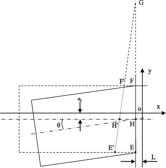
Analysis of plate movement at the entry side.

Assume that the rigid body rotation angular velocity of the rolled piece in the entry side is ω_H, the radius of curvature corresponding to the camber of the rolled piece is ρ_H(ρ_H = GH). The formula can be obtained from the plane motion theory of rigid body as follows.   

$$\{\begin{array}{l}{v}_E=-\left(-{\rho }_H+\frac{W}{2}\right)\times {\omega }_H=\left({\rho }_H-\frac{W}{2}\right)\times {\omega }_H\\ v_F=-\left(-{\rho }_H-\frac{W}{2}\right)\times {\omega }_H=\left({\rho }_H+\frac{W}{2}\right)\times {\omega }_H\end{array}$$(3)

Where W is the width of the rolled piece at the entrance of the deformation zone, mm.   

$$\{\begin{array}{l}{\rho }_H=W\times {\overline{v}}_H/\mathrm{\Delta }{v}_H\\ {\omega }_H={\overline{v}}_H/{\rho }_H\\ {\overline{v}}_H=(v_E+v_F)/2\\ \mathrm{\Delta }{v}_H=v_F-v_E\end{array}$$(4)

Where ${\overline{v}}_H$ is average velocity of entry rolled piece, m/s; Δv_H is entry velocity difference on both sides of rolled piece, m/s. In time interval of Δt, the rotation angle of the piece around the velocity instantaneous center in the entry side is denoted as Δθ, the distance between the center line of the rolled piece and the center line of the rolled piece is Δa, then   

$$\{\begin{array}{l}\mathrm{\Delta }\theta ={\omega }_H\times \mathrm{\Delta }t\\ \mathrm{\Delta }\alpha ={\rho }_H\left(cos\mathrm{\Delta }\theta -1\right)\\ \theta =\sum \mathrm{\Delta }\theta \\ \alpha =\sum \mathrm{\Delta }\alpha \end{array}$$(5)

Where a is the offset of the entry piece, mm; θ is the total deflection Angle of the entry piece, rad.

2.3. Setting Model of Rolling Piece Camber Control

According to the principle of constant volume flow in the rolling process, it is assumed that the metal does not flow horizontally during the rolling process, that is, the width of the rolled piece remains unchanged. When the rolling state of the rolled piece is not symmetrical, the following equation can be obtained from the volume flow increment equation.²¹⁾   

$$\frac{\mathrm{\Delta }H}{H}+\frac{\mathrm{\Delta }{v}_H}{{\overline{v}}_H}=\frac{\mathrm{\Delta }h}{h}+\frac{\mathrm{\Delta }{v}_h}{{\overline{v}}_h}$$(6)

Where H is average thickness of the entry rolled piece, mm; h is average thickness of the exit rolled piece, mm; ΔH is the thickness difference between the two sides of the entry rolled piece, mm; Δh is the thickness difference between the two sides of the exit rolled piece, mm.

From Eqs. (1), (2) and (6), the relation model between the radius of curvature at the entry and exit of the rolled piece and the difference of the wedge rate of the rolled piece can be obtained.   

$$\{\begin{array}{l}{\displaystyle \frac{1}{{\rho }_h}}={\displaystyle \frac{1}{{\rho }_H}}-{\displaystyle \frac{\mathrm{\Delta }\psi }{W}}\\ \mathrm{\Delta }\psi ={\displaystyle \frac{\mathrm{\Delta }h}{h}}-{\displaystyle \frac{\mathrm{\Delta }H}{H}}\end{array}$$(7)

Where Δψ is the difference of the wedge rate of the entry and exit rolled piece, mm; ρ_H is the radius of curvature at the entry of the rolled piece, mm; ρ_h is the radius of curvature at the exit of the rolled piece, mm.

In order to reduce the camber of the exit rolling piece, the wedge of the exit rolling piece is usually satisfied by setting the adjustment value of the roll gap inclination in advance, to carry out feedforward control on the camber of the rolled piece.

Therefore, the radius of the curvature of the exit rolled piece is set as ρ_h = ∞, the mathematical model of feedforward control for rolling piece camber can be represented as   

$$\mathrm{\Delta }h=h\times \left[\frac{W}{{\rho }_H}+\frac{\mathrm{\Delta }H}{H}\right]$$(8)

If the curvature radius ρ_H of the entry rolling piece is measured through the rolling piece camber detection system, then the section shape parameter ΔH/H of the entrance rolling piece is calculated by using the online data of rolling force and roll gap obtained from the last pass. At the same time, the exit thickness h of the rolled piece can be predicted according to the setting of the pass gap and the rolling force prediction model. Using the camber feedforward control model, the target wedge of the exit piece can be obtained. Then the influence function method is used to calculate the setting values of the slope adjustment of the roll gap, and send to HGC system to adjust the roll gap on both sides.

The rigid tilt quantity of the roll system is the differential value of the roller seam of the mill drive and the non-drive side, and the basic equation of the rigid tilt of the roll is:   

$$\mathrm{\Delta }S=\frac{P_{DS}}{K_{DS}}-\frac{P_{NDS}}{K_{NDS}}+\mathrm{\Delta }{S}_0=\frac{P_{DS}\times K_{NDS}-P_{NDS}\times K_{DS}}{K_{DS}\times K_{NDS}}+\mathrm{\Delta }{S}_0$$(9)

Where ΔS is rigid tilt of roll system, mm; ΔS₀ is no-load roll gap inclination, mm; P_DS is the pressure of the drive side of the back-up roller, kN; P_NDS is the pressure of the non-drive side of the back-up roller, kN; K_DS is rolling mill rigidity of drive side, kN/mm; K_NDS is rolling mill rigidity of non-drive side, kN/mm.   

$$\begin{array}{l}\mathrm{\Delta }h=h_{DS}-h_{NDS}=\mathrm{\Delta }S\times {\displaystyle \frac{W}{L_B}}+{\displaystyle \frac{8\times W\times \mathrm{\Delta }W\times C_R}{L_W^2}}\\ \hspace{1em}\hspace{0.5em}={\displaystyle \frac{W}{L_B}}\times \left[{\displaystyle \frac{2\times (P_{DS}-P_{NDS})\times K-(P_{DS}+P_{NDS})\times \mathrm{\Delta }K}{2\times K^2-0.5\times \mathrm{\Delta }{K}^2}}\right]\\ \hspace{1em}\hspace{1em}+{\displaystyle \frac{W}{L_B}}\times \mathrm{\Delta }{S}_0+{\displaystyle \frac{8\times W\times \mathrm{\Delta }W\times C_R}{L_W^2}}\end{array}$$(10)

Where h_DS is rolled piece thickness of drive side, mm; h_NDS is rolled piece thickness of non-drive side, mm; C_R is work roll crown, mm; ΔW is distance from centerline of steel plate, mm; K is the average stiffness mill, kN/mm; ΔK is the difference of the stiffness on both sides of mill, kN/mm. L_B is the length of work roll body, mm; L_W is the length of backup roll body, mm.

3. A Camber Feedback Model Based on Machine Vision

There are many influencing factors of rolling piece camber and they are coupled with each other. For plate camber caused by other asymmetric influencing factors that cannot be accurately determined in advance, the control effect is not ideal. Moreover, feedforward control has high requirements on the calculation and measurement accuracy of variables such as thickness and wedge, and having long lag time, which makes it difficult to be realized. Therefore, it is hard to satisfy the actual production requirements by simply relying on feedforward control. In this paper, based on the quadratic parabola distribution of roll crown and the assumption of roll rigidity model, a feedback control model applicable to different factors was established to compensate the deficiency of feedforward control of roll straightness as be shown in Fig. 3.

Fig. 3.

The camber feedback control of plate based on parameter correction. (Online version in color.)

The purpose of establishing a rolling piece camber detection system is to obtain quantitatively the information of the rolled piece bending degree that may be produced in the rolling process. The camber information obtained in this paper will eventually be used in the subsequent development and calculation of the camber control model, so the curvature representation method is used to measure the bending degree of the rolled piece.

The machine vision device was installed 1850 mm from the downstream of the mill. With machine vision method, the subpixel coordinates of the rolled piece edges can be obtained, and the size of the plan view of rolled piece can also be settled indirectly. But curvature calculation results on the both sides of the rolled piece are different due to inconsistent width of rolled piece, which is not conducive to the input variables of subsequent camber control model, so the midline curvature is represented as the curvature of the entire rolled piece as be shown in Fig. 4.

Fig. 4.

The diagram of the rolling center line. (Online version in color.)

It can be seen from the Fig. 4 that the center line of the rolling piece, which should have been vertical, became a section of arc under the action of side bending, and due to the asymmetry in the process of rolling conditions and external environment, the influence of the shape of the rolled piece scoliosis can’t present a regular arc, which along the direction of each point has some difference. At the same time, after image preprocessing, most of the isolated points and noise points have been basically filtered out. Therefore, we use the least square optimization algorithm with minimum time and space complexity to fit the center line to calculate the curvature radius of the rolled piece.

The basic idea of circle fitting method based on least square algorithm is to use a section of arc to describe the middle line of rolled piece, that is, to find a circle so that the subpixel coordinate points on the middle line of the rolled piece are mostly on this circle. The radius of the circle is the radius of the rolled piece camber and the curvature of a circle is the curvature of the rolled piece camber, which is achieved by minimizing the squared residuals of the appropriate sample points. The curve equation of a circle in a two-dimensional coordinate plane is represented as   

$${(x-a)}^2+{(y-b)}^2=r^2$$(11)

The residual equation of Eq. (10) is   

$${\epsilon }_i={(x_i-a)}^2+{(y_i-b)}^2-r^2$$(12)

Where i=1,2,...,S; S is maximum number of subpixel coordinate points of the middle line of the rolled piece; (x_i,y_i) is the subpixel coordinate of the center line; (a,b) is center coordinates of the fitted circle; r is the radius of the fitted circle.

If the error distance is substituted for the number distance, then the sum of squared residuals is   

$$Q=\sum _{i=0}^{i<s}{\epsilon }_i^2={\sum _{i=0}^{i<s}\left[{(x_i-a)}^2+{(y_i-b)}^2-r^2\right]}^2$$(13)

Based on the extremum principle of least square method, the residual squared sum is minimized and the following equation can be obtained.   

$$\frac{\partial Q}{\partial a}=\frac{\partial Q}{\partial b}=\frac{\partial Q}{\partial r}=0$$(14)

Simultaneous Eqs. (11), (12) and (13)   

$$\{\begin{array}{l}{a}^2-2\overline{x}a+b^2-2\overline{y}b-r^2+\overline{x^2}+\overline{y^2}=0\\ \overline{x}{a}^2-2\overline{x^2}a+\overline{x}{b}^2-2\overline{x}\overline{y}b-\overline{x}{r}^2+\overline{x^3}+\overline{x}\overline{y^2}=0\\ \overline{y}{a}^2-2\overline{x}\overline{y}a+\overline{y}{b}^2-2\overline{y^2}b-\overline{y}{r}^2+\overline{x^2}\overline{y}+\overline{y^3}=0\end{array}$$(15)

Where $\overline{x^m}\overline{y^n}=\sum _{i=0}^{i<s}{x}_i^m{y}_i^n/\sum _{i=0}^{i<s}i$.

It can be seen from the above formulas that the method of least square circle fitting is used to fit the middle line of rolled piece and calculate the average curvature of rolled piece camber. Although the form of the method is complex, the curvature can be accurately calculated by circulating the subpixel coordinate points of the rolled piece middle line all at once. The calculation accuracy is not high and the calculating quantity can be reduced significantly. In order to improve the computing speed, data points can be selected discretely in the process of solving the algorithm, subpixel coordinate points which evenly distributed on the middle line of the rolled piece are collected as sample points to realize the information extraction of rolled pieces.

Based on the above principles and methods, the midpoint of the edge subpixel coordinate of the rolled piece is taken as the midline coordinate, then extract 50 points which is evenly distributed on the middle line of the rolled piece and substitute them into the above formula for circle fitting. The average bending curvature of the rolled piece is 1.52943×10⁻⁴mm⁻¹, the sum of squares due to error (SSE) is 1.601 and the fitting degree is 0.91142, The fitting effect is shown in Fig. 5.

Fig. 5.

The fitting map of the camber midline. (Online version in color.)

Due to different rolling pieces and different rolling passes when camber occurs, the bending degree of rolling pieces is different, therefore, in order to verify the robustness of our algorithm, we use a 3500 mm plate mill as an application example and check the camber of the rolling piece at the exit of the mill (Fig. 6).

Fig. 6.

The change of camber rate of the exit rolling plate. (Online version in color.)

As can be seen in the Fig. 6, during the rolling process, the whole rolled piece bends to the operating side, and the shape of the rolled piece is “M”, That is that the bending degree of the rolled piece increases first, then decreases, and then increases, which is consistent with the actual rolling piece shape change. The wedge rate is the ratio between wedge rate and average thickness of the rolled piece. The premise that produces camber is that the wedge rate of the rolled piece at the entry and exit changes. Therefore, the rolled piece camber at the exit side has a great relationship with the change of the wedge rate of the rolled piece.

According to the basic theory of metal plastic deformation, the distribution equation of rolling force per unit width can be established according to the thickness of rolled piece and the distribution equation of plastic stiffness of rolled piece by taking the middle part of rolled piece as the origin.   

$$\begin{array}{l}p(x)=\left[H(x)-h(x)\right]\times M(x)=(H-h)\times M\\ \hspace{1em}\hspace{1em}\hspace{0.5em}+{\displaystyle \frac{(\mathrm{\Delta }H-\mathrm{\Delta }h)\times M+(H-h)\times \mathrm{\Delta }M}{W}}\times x\\ \hspace{1em}\hspace{1em}\hspace{0.5em}+{\displaystyle \frac{(\mathrm{\Delta }H-\mathrm{\Delta }h)\times \mathrm{\Delta }M}{W^2}}\times x^2\end{array}$$(16)

The force balance equation of the roll system can be established according to the distribution equation of rolling force per unit width based on the rolling force, the bending force F_W and the press force of the screw or hydraulic cylinder on both sides of the supporting roller.   

$$\begin{array}{l}{P}_{DS}+P_{NDS}=2\times F_W+{\int }_{-W/2}^{W/2}\left[p(x)\right]dx=\\ {\displaystyle \frac{24\times F_W+12\times W\times (H-h)\times M+W\times (\mathrm{\Delta }H-\mathrm{\Delta }h)\times \mathrm{\Delta }M}{12}}\end{array}$$(17)

The rolling piece deviation is the deviation between the center line of rolling piece and the rolling center line, and the rolling piece deviation towards the transmission side is defined as positive value. Taking the rolling center line as the base point and combining with the distribution equation of rolling force per unit width, the torque balance equation of the roll system can be obtained as follows:   

$$\begin{array}{l}(P_{DS}+P_{NDS})\times \frac{L_B}{2}={\int }_{-W/2}^{W/2}\left[p(x)\times (\mathrm{\Delta }W+x)\right]dx=\\ \frac{W}{12}\times [12\times M\times (H-h)\times \mathrm{\Delta }W+(\mathrm{\Delta }H-\mathrm{\Delta }h)\times \mathrm{\Delta }M\\ \hspace{1em}\mathrm{\hspace{0.17em} }\times \mathrm{\Delta }W+W\times (\mathrm{\Delta }H-\mathrm{\Delta }h)\times M+W\times (H-h)\times \mathrm{\Delta }M]\end{array}$$(18)

Then,   

$$\begin{array}{l}(P_{DS}+P_{NDS})=\\ \frac{W}{6\times L_B}\times [12\times M\times (H-h)\times \mathrm{\Delta }W+(\mathrm{\Delta }H-\mathrm{\Delta }h)\times \mathrm{\Delta }M\\ \hspace{1em}\hspace{1em}\mathrm{\hspace{0.17em} }\mathrm{\hspace{0.17em} } \times \mathrm{\Delta }W+W\times (\mathrm{\Delta }H-\mathrm{\Delta }h)\times M+W\times (H-h)\times \mathrm{\Delta }M]\end{array}$$(19)

Where L_B is press down screw or hydraulic cylinder center distance on both sides of mill.

Substitute Eqs. (18) and (19) into Eq. (10), then the exit mill wedge Δh can be obtained from simultaneous solution of the force balance equation, the moment balance equation, and the wedge equation.   

$${\displaystyle \{\begin{array}{l}\mathrm{\Delta }h=a_1\times \mathrm{\Delta }H+a_2\times \mathrm{\Delta }M+a_3\times \mathrm{\Delta }K+a_4\times \mathrm{\Delta }W+a_5\times \mathrm{\Delta }{S}_0\\ a_1={\displaystyle \frac{4\times K\times M\times W^3}{6\times L_B^2\times (4\times K^2-\mathrm{\Delta }{K}^2)+4\times K\times M\times W^3+W^2\times (4\times K\times \mathrm{\Delta }W-L_B\times \mathrm{\Delta }K)\times \mathrm{\Delta }M}}\\ a_2={\displaystyle \frac{4\times K\times W^3\times (H_0-h_0)+W^2\times (4\times K\times \mathrm{\Delta }W\times \mathrm{\Delta }H-L_B\times \mathrm{\Delta }H\times \mathrm{\Delta }K)}{6\times L_B^2\times (4\times K^2-\mathrm{\Delta }{K}^2)+4\times K\times M\times W^3+W^2\times (4\times K\times \mathrm{\Delta }W-L_B\times \mathrm{\Delta }K)\times \mathrm{\Delta }M}}\\ a_3=-{\displaystyle \frac{12\times L_B\times W\times [(W\times (H_0-h_0)\times M_0+2\times F_W]}{6\times L_B^2\times (4\times K^2-\mathrm{\Delta }{K}^2)+4\times K\times M\times W^3+W^2\times (4\times K\times \mathrm{\Delta }W-L_B\times \mathrm{\Delta }K)\times \mathrm{\Delta }M}}\\ a_4={\displaystyle \frac{48\times K\times W^2\times M_0\times (H_0-h_0)+48\times W\times (4\times K^2-\mathrm{\Delta }{K}^2)\times {(L_B/L_W)}^2\times C_R}{6\times L_B^2\times (4\times K^2-\mathrm{\Delta }{K}^2)+4\times K\times M\times W^3+W^2\times (4\times K\times \mathrm{\Delta }W-L_B\times \mathrm{\Delta }K)\times \mathrm{\Delta }M}}\\ a_5={\displaystyle \frac{6\times W\times L_B\times (4\times K^2-\mathrm{\Delta }{K}^2)}{6\times L_B^2\times (4\times K^2-\mathrm{\Delta }{K}^2)+4\times K\times M\times W^3+W^2\times (4\times K\times \mathrm{\Delta }W-L_B\times \mathrm{\Delta }K)\times \mathrm{\Delta }M}}\end{array}}$$(20)

The difference of the wedge rate can be calculated as:   

$$\begin{array}{l}\mathrm{\Delta }\psi =\mathrm{\Delta }h/h-\mathrm{\Delta }H/H\\ =\frac{1}{h}\times \left[(a_1-1/\lambda )\times \mathrm{\Delta }H+a_2\times \mathrm{\Delta }M+a_3\times \mathrm{\Delta }K+a_4\times \mathrm{\Delta }W+a_5\times \mathrm{\Delta }{S}_0\right]\end{array}$$(21)

Where λ is reduction coefficient, λ = H/h.

Substitute Eq. (21) into Eq. (7)   

$$\begin{array}{l}{\displaystyle \frac{1}{{\rho }_h}}={\displaystyle \frac{1}{{\rho }_H}}-{\displaystyle \frac{\mathrm{\Delta }\psi }{W}}={\displaystyle \frac{1}{{\rho }_H}}-{\displaystyle \frac{1}{W\times h}}\\ \times \left[(a_1-1/\lambda )\times \mathrm{\Delta }H+a_2\times \mathrm{\Delta }M+a_3\times \mathrm{\Delta }K+a_4\times \mathrm{\Delta }W+a_5\times \mathrm{\Delta }{S}_0\right]\end{array}$$(22)

Roll tilt control is usually used to adjust the camber of plate, therefore, in order to improve or eliminate the camber defect of rolled piece, the curvature radius ρ_h of the exit piece can be approached to infinity. According to the basic theory of plate and strip rolling, the equations of bite angle, neutral angle, forward slip value and inlet and outlet velocity are shown by the following equations.   

$$\{\begin{array}{l}\alpha =\sqrt{(H-h)/R_W}\\ \gamma =\alpha /2\\ S_h={\displaystyle \frac{{\gamma }^2\times R_W}{h}}={\displaystyle \frac{H-h}{4\times h}}\\ v_h=(1+S_h)\times v_R\\ v_H={\displaystyle \frac{h\times (1+S_h)\times v_R}{H}}\end{array}$$(23)

Where α is bite angle; γ is neutral angle; S_h is forward slip value; R_W is work roll radius, mm; v_R is work roll speed, mm/s.

Substitute Eq. (23) into Eqs. (1) and (4), then the speed difference between the entry and exit on both sides of the rolled piece can be calculated by the following equations.   

$$\{\begin{array}{l}\mathrm{\Delta }{v}_h=v_{h\_A}-v_{h\_B}={\displaystyle \frac{H_A\times h_B-H_B\times h_A}{4\times h_A\times h_B}}\times v_R\hfill \\ \mathrm{\Delta }{v}_H=v_{H\_E}-v_{H\_F}={\displaystyle \frac{3\times (H_F\times h_E-H_E\times h_F)}{4\times h_E\times h_F}}\times v_R\hfill \end{array}$$(24)

According to Eqs. (1) and (4), the contracted relationship between the curvature radius of the exit and the entry workpiece is shown as follows.   

$$\{\begin{array}{l}{\displaystyle \frac{{\rho }_h}{{\rho }_H}}=\lambda \times {\displaystyle \frac{\mathrm{\Delta }{v}_H}{\mathrm{\Delta }{v}_h}}=-{\displaystyle \frac{3\lambda \times (4h^2-\mathrm{\Delta }{h}^2)}{4H^2-\mathrm{\Delta }{H}^2}}\approx -{\displaystyle \frac{3}{\lambda }}\hfill \\ {\displaystyle \frac{1}{{\rho }_h}}-{\displaystyle \frac{1}{{\rho }_H}}={\displaystyle \frac{1}{{\rho }_h}}\times \left[1+{\displaystyle \frac{1}{\lambda }}\right]\hfill \end{array}$$(25)

Where λ is coefficient of reduction, λ = H/h.

The relationship of the curvature radius of the entry and exit rolled pieces is substituted into Eq. (22), and the mathematical model of the feedback control of the rolled pieces camber involving the adjustment value of the loaded roll gap and the radius of the camber curvature is shown in Eq. (25).   

$$\begin{array}{l}\mathrm{\Delta }S\prime =-{\displaystyle \frac{h}{{\rho }_h}}\times {\displaystyle \frac{W}{a_5}}\times \left[1+{\displaystyle \frac{3}{\lambda }}\right]-{\displaystyle \frac{(a_1-1/\lambda )}{a_5}}\times \mathrm{\Delta }H-{\displaystyle \frac{a_2}{a_5}}\\ \hspace{1em}\hspace{1em}\times \mathrm{\Delta }M-{\displaystyle \frac{a_3}{a_5}}\times \mathrm{\Delta }K-{\displaystyle \frac{a_4}{a_5}}\times \mathrm{\Delta }W\end{array}$$(26)

Where ΔS′ is roll tilt adjustment of rolling mill, mm; ΔM is plastic coefficient difference between two sides of rolled piece, kN/mm; ΔW is offset of center line of rolled piece relative to center line of rolled piece, mm; ΔH is wedge of inlet piece, mm.

4. Prediction Model of Camber Synthesis Leveling Based on PSO-LSSVM Algorithm

Based on the above models, the required tilt adjustment value of the load roll gap of the mill can be calculated according to the detected camber value, to carry out feedback control on the camber defect. If the bending degree can be predicted by the model before the detection result of the camber, then the tilt value of the roll gap can be controlled in advance to avoid the occurrence of side bend. In the process of measuring camber with machine vision, a lot of production data are produced under different products and working conditions. Intelligent optimization algorithm can be used to predict the plate camber, and the corresponding online comprehensive leveling control model and control strategy can be established to optimize the adjustment value of the roll slot and to achieve the high-precision intelligent control of the plate camber.

4.1. Principle of LSSVM

Least Squares Support Vector Machines (LSSVM) evolves from standard support vector machines (SVM) to deal with the complex problems of classification and regression in practice, and it is widely used in pattern recognition and nonlinear function estimation. So LSSVM is a good choice to predict the plate camber.

The training sample set is defined as (x_k,y_k),k=1,2,...,N, where x_k∈R^d and it is the input vector for the k sample; y_k∈R^d and it is the measured output value for the k sample,

The LSSVM regression problem has the same form as the SVM regression problem, which can be constructed the optimal regression function f(x)=w^Tφ(x)+b in the high dimensional eigenspace by nonlinear mapping. f(x) can be correctly fitted the output vector corresponding to the unknown input vector with the lowest error. The constraint condition of the SVM problem is the inequality constraint equation.   

$$\begin{array}{l}\underset{w,b,\xi }{min}{J}_p(w,\xi )=\frac{1}{2}{w}^{T}w+c\sum _{k=1}^N({\xi }_k+{\hat{\xi }}_k)\hfill \\ s.t.\mathrm{\hspace{0.17em} } y_k-w^T\phi (x_k)-b\le \epsilon +{\xi }_k,\hfill \\ \hspace{1em}\mathrm{\hspace{0.17em} }{w}^T\phi (x_k)+b-y_k\le \epsilon +{\hat{\xi }}_k,\mathrm{\hspace{0.17em} } k=1,\mathrm{...},N.\hfill \\ {\hat{\xi }}_k\ge 0,{\xi }_k\ge 0,\mathrm{\hspace{0.17em} } k=1,\mathrm{...},N.\hfill \end{array}$$(27)

Where w is the normal vector of the hyperplane; b is the intercept of the hyperplane; ξ_k and ${\hat{\xi }}_k$ are slack variables; ε is a hyperparameter that determines the width of the interval boundary; c is regularization coefficient. Classification is finding a separated hyperplane between input vectors, and LSSVM regression uses hyperplane to fit the input vector, whose common goal is to find an optimal hyperplane, so they have the same target function. The constraints can be replaced by equality constraints, and the corresponding optimization equation of LSSVM regression problem can be obtained as shown in Eq. (28).   

$$\begin{array}{l}\underset{w,b,\mathrm{l}}{min}{J}_p(w,\mathrm{𝓁})=\frac{1}{2}{w}^{T}w+\gamma \frac{1}{2}\sum _{k=1}^N{\mathrm{𝓁}}_k^2\\ s.t.\mathrm{\hspace{0.17em} } y_k=w^T\phi (x_k)+b+{\mathrm{𝓁}}_k,\mathrm{\hspace{0.17em} } k=1,\mathrm{...},N\end{array}$$(28)

Then, Lagrange multiplier method is adopted for Eq. (28), and Eq. (29) can be obtained.   

$$L(w,b,\mathrm{𝓁},\alpha )={\mathrm{J}}_{\mathrm{p}}(w,\mathrm{𝓁})-\sum _{k=1}^N{\alpha }_k\left\{w^T\phi (x_k)+b+{\mathrm{𝓁}}_k-y_k\right\}$$(29)

And take the partial derivatives of w,b,ℓ_k,α_k.   

$$\{\begin{array}{l}{\displaystyle \frac{\partial L}{\partial w}}=0\to w=\sum _{k=1}^N{\alpha }_k\phi (x_k)\hfill \\ {\displaystyle \frac{\partial L}{\partial b}}=0\to w=\sum _{k=1}^N{\alpha }_k=0\hfill \\ {\displaystyle \frac{\partial L}{\partial {\mathrm{l}}_k}}=0\to {\alpha }_k=\gamma {\mathrm{𝓁}}_k,\mathrm{\hspace{0.17em} } k=1,\mathrm{...},\mathrm{N}.\hfill \\ {\displaystyle \frac{\partial L}{\partial {\alpha }_k}}=0\to w^T\phi (x_k)+b+{\mathrm{𝓁}}_k-y_k=\text{0},\mathrm{\hspace{0.17em} } k=1,\mathrm{...},\mathrm{N}.\hfill \end{array}$$(30)

By writing Eq. (30) as a matrix form and then omitting w and ℓ through transformation, and introducing Mercer condition, the dimensional linear equations for solving a and b are shown in Eq. (31).   

$$\left(\begin{array}{cc}0& l_v{}^T\\ l_v& \mathrm{\Omega }+I/\gamma \end{array}\right)\left(\begin{array}{l}b\\ \alpha \end{array}\right)=\left(\begin{array}{l}0\\ y\end{array}\right)$$(31)

Where y=[y₁;...;y_N]; α=[α₁;...;α_N]; l_v=[1,1,...,1]^T; A=Ω+I/γ; I is the identity matrix; Ω is the kernel matrix, its definition is as follows.   

$${\mathrm{\Omega }}_{kl}=\phi {(x_k)}^T\phi (x_l)=K(x_k,x_l)\hspace{1em}k,l=1,\mathrm{...},N$$(32)

Finally, the regression model of LSSVM is solved as shown in Eq. (33).   

$$f(x)=\sum _{k=1}^N{\alpha }_{k}K(x,x_k)+b$$(33)

Where K is the kernel function; α_k=A⁻¹(y−bl_v); $b=\frac{l_v{}^T{A}^{-1}y}{l_v{}^T{A}^{-1}{l}_v}$.

4.2. Principle of PSO

PSO was proposed by Kennedy and Eberhart in 1995, which originated from the study of bird predation behavior. Group iteration and search are used to find the optimal solution through the evolution from disorder to order in the solution space. The particle has only two properties: velocity v and position x. Velocity represents the speed of movement and position represents the direction of movement. Each particle searches the optimal solution separately in the search space, and its extreme value is recorded as the current individual extremum P_best, the individual extremum is shared with other particles in the whole particle swarm. In this way, the current global optimal solution G_best of the entire particle swarm is found. All particles in the particle swarm adjust their velocity and position according to the current individual extremum P_best found by themselves and the current global optimal solution G_best shared by the whole particle swarm. The whole process is divided into: initialize particle swarm; evaluate particle; calculate fitness value; find individual extremum; find global optimal solution; modify the velocity and position of particle, and the update formula for velocity and position during optimization are as follows   

$$v_{id}(t+1)=w.v_{id}(t)+c_1.r_1(p_{id}-x_{id}(t))+c_2.r_2(p_{gd}-x_{id}(t))$$(34)

  

$$x_{id}(t+1)=x_{id}(t)+v_{id}(t+1)\hspace{1em}(1\le i\le m,1\le d\le D)$$(35)

Where i is number of the particle; d is dth dimensional component of particle i; t is the number of the particles iterations; v_id is dth dimensional component of the flight velocity vector when the ith particle is adjusted, v_id∈[v_min,v_max]; p_id is dth dimensional component of global extremum; p_gd is dth dimensional component of individual extremum; w is inertia factor, which is used to regulate the ability to search the solution space; r₁, r₂ is an uniformly distributed random number between 0 and 1; c₁, c₂ are learning factors.

Through the analysis of the above formulas, we find that the particle velocity during dynamic adjustment is mainly composed of three parts: The first part is the initial velocity vector of the particle, which enables the particle to have global searching ability, also known as memory term; The second part is a vector from the initial point to the individual extreme value point, which can be understood as the judgment made by the particle to reduce the error through its own experience, also known as its own cognitive term. The third part is a vector from the initial point to the global extreme point, which reflects the interaction and information sharing between particles, to determine their own direction of motion according to the experience of peers, also known as group cognitive term. the schematic diagram of particle position and velocity adjustment in two-dimensional space during iteration is presented is Fig. 7.

Fig. 7.

The Schematic of particle iteration.

4.3. LSSVM Algorithm Based on PSO Parameter Optimization

After the above research and analysis, the complex nonlinear relationship between the side bending of rolled pieces and the influencing factors is considered, LSSVM regression model with RBF as kernel function is used to control the plate camber during rolling. Experience shows that different values of critical coefficient α_c, kernel width coefficient σ and penalty coefficient γ will lead to great differences in the performance of LSSVM models, which only affects the approximation ability of the model, and the accuracy of the model is usually determined according to the actual situation.

Therefore, in order to improve the learning accuracy and generalization performance of the LSSVM regression model, we combined the particle swarm optimization algorithm (PSO) with the least-squares support vector machine (LSVM), and used PSO algorithm to optimize the search of the least-squares support vector machine parameters (penalty factor and kernel parameters), to establish the PSO-LSSVM model of rolling piece camber leveling. The specific process of its algorithm is as follows (Fig. 8).

Fig. 8.

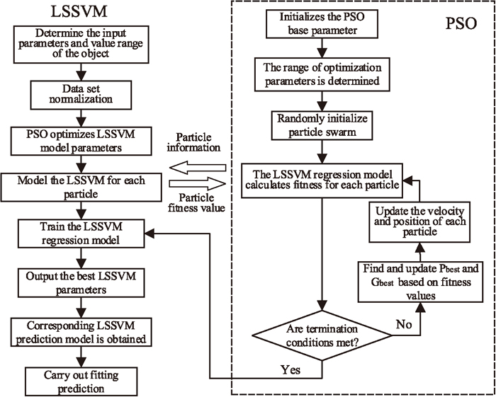
The flow chart of super parameters selection based on particle swarm optimization algorithm.

5. Results and Discussion

In order to reduce the frequency of camber in plate rolling process, we need to analyze the camber law under different working conditions. Taking a 3500 mm plate mill in China as an example and carrying out the research work to the change rule of camber, the main technical parameters of plate mill is shown in Table 1.

Table 1. The main technical parameters of roughing mill.

Technical parameter	Parameter range	Technical parameter	Parameter range
Work roll size	φ950/1050×3500 mm	Zero Rolling force	22700 kN
Work roll crown	−150 μm	Rolling speed	0–6.6 m/s
Center distance of bending cylinder	5040 mm	Press down mode	Electric & hydraulic
Backup roll size	φ1900/2100×3300 mm	Mill stiffness	8100 kN/mm
Backup roll crown	0	Maximum rolling force	70000 kN
Main motor power	7000 kW×2	Maximum rolling torque	3500 kN.m×2

The raw steel Q420C was used as the research object, slab width is 2000 mm, slab thickness is 250 mm, target width of production is 2800 mm, target thickness of product is 10 mm, 20 mm and 30 mm respectively. Based on the above equipment parameters, the curvature change law with different thickness of plate, wedge of plate, reduction of plate and roll tilt Angle was studied from the calculation results of Eqs. (1), (2), (7) and (8) as be shown in Figs. 9, 10, 11, 12.

Fig. 9.

Plate curvature with different thickness and wedge. (Online version in color.)

Fig. 10.

Plate curvature with different reduction and wedge. (Online version in color.)

Fig. 11.

Plate curvature with different roll tilt Angle and thickness. (Online version in color.)

Fig. 12.

Plate curvature with different roll tilt Angle and reduction. (Online version in color.)

It can be seen from Fig. 9 that the thinner is the thickness of the steel plate, the greater is the contribution of the wedge to plate curvature. When the thickness is equal to 10 mm and the wedge of the entry steel plate is 4 mm, plate curvature can be up to 1.44×10⁻⁴mm⁻¹. Figure 10 illustrates that if the entry thickness equals to 30 mm, the bigger is the reduction of the steel plate, the greater is the contribution of the wedge to plate curvature. Nevertheless, the maximum camber of exit plate is only 0.5×10⁻⁴mm⁻¹, which means that the camber curvature of thicker steel plate is not sensitive to the plate wedge. Figure 11 shows that the thinner is the thickness of the steel plate, the greater is the contribution of the roll tilt Angle to plate curvature. When the thickness is equal to 10 mm and the roll tilt Angle of the entry steel plate is 0.4°, plate curvature can be up to 3.946×10⁻⁴mm⁻¹. If the thickness reduction of 30 mm steel plate is set up as 10 mm, the curvature can reach 3.67×10⁻⁴mm⁻¹ when the tilt Angle is 0.4 as be shown in Fig. 12.

Figures 11 and 12 illustrate that the roll tilt Angle is very sensitive to changing the camber curvature. If the intelligent algorithm can accurately predict the curvature and change law of the plate camber before the steel plate entering the rolling mill, the equations mentioned above can be used to calculate and control the roll tilt angle, so plate camber prediction becomes an important task.

Based on camber detection system, a wealth of data has been provided. In this paper, a PSO-LSSVM based side bend prediction model is established. In order to meet the needs of actual field production, many field production data can be used to train the camber model. Before machine learning model training, in order to improve the accuracy of model training, it is necessary to select and extract features of data. Feature selection and extraction are of great importance to machine learning model. Feature selection has a clear and definite relationship with the research object, as well as features with clear physical meaning and conciseness. Moreover, dimensionality reduction treatment of features is of great significance for obtaining a higher precision rolling mill roll slot inclination adjustment value model. At the same time, it should be noted that the selected features should be easy to understand, which have a great influence on the research objects and can be detected or calculated indirectly in actual production.

500 set of actual production data were collected under different working conditions and different product conditions. 250 set of data were used for building and training a PSO-LSSVM based on comprehensive prediction model of rolling piece camber, the remaining 250 set of data were used to verify the calculation accuracy of the model established. Curvature comparison of PSO-LSSVM, BP neural network and measured data of training and testing are given in Figs. 13 and 14. Figures 15 and 16 demonstrates the percentage error deviations of predicted curvatures using PSO-LSSVM and BP neural network. The difference of prediction accuracy between the two models cannot be seen intuitively from Figs. 13 and 14. So, the relative error in the prediction models are chosen to be compared. Figures 15 and 16 shows clearly the difference between the relative error indices of PSO-LSSVM and BP neural network models from training data and testing data. For BP neural network model, the relative error of curvature prediction is larger than that of PSO-LSSVM model, the reference range is y = ±20% and most of the samples are in error range. However, there are scattered outliers whose relative errors exceed ±20% of the error lines. The prediction effect of curvature based on PSO-LSSVM model is obviously better than that of BP neural network model, the relative error is within ±5% of both the training set and the testing set.

Fig. 13.

The comparison chart of training effects of PSO-LSSVM model. (Online version in color.)

Fig. 14.

The comparison chart of testing effects of PSO-LSSVM model. (Online version in color.)

Fig. 15.

The training set relative error of the models. (Online version in color.)

Fig. 16.

The testing set relative error of the models. (Online version in color.)

Based on PSO-LSSVM model, the plate camber can be predicted accurately with actual production data. The mathematical model of roll gap tilt adjustment (Eq. (25)) can be used to achieve the goal of improving or eliminating the lateral bending of export rolled pieces. To test the generalization performance of the PSO-LSSVM model, it is necessary to collect the data of steel plates without camber after the roll tilt adjustment for different processes and product specification, combining with the field data, the 250 set of test sample data are input to the PSO-LSSVM forecasting model. Contrast figure of calculated values and measure values of curvature is given in Fig. 17.

Fig. 17.

The comparison of measured values and calculated values of PSO-LSSVM model. (Online version in color.)

Figure 17 shows that the relative error range of curvature value is within ±6% after being compensated by PSO-LSSVM algorithm, and these data are collected on the premise that the final product has good straightness. The method adopted in this paper can enrich and perfect the theory and method of side bend control of rolling pieces, which has important theoretical and practical guiding significance to field production.

6. Conclusions

(1) Based on the basic equation of transverse asymmetric rolling, a mathematical model of plate camber curvature radius of the exit side and entry side is investigated. In order to reduce the camber of the exit rolling piece, the mathematical model of feedforward control for rolling piece camber is represented.

(2) A machine vision method for camber measuring is adopted in which the subpixel coordinates of the rolled piece edges can be obtained, and the size of the plan view of rolled piece can also be settled indirectly so as to carry out feedback control on the camber defect.

(3) Tilt value of the roll gap can be controlled in advance to avoid the occurrence of camber which predicted with high accuracy. A prediction model of camber synthesis leveling based on PSO-LSSVM algorithm is used, the relative error is within ±5% of both the training set and the testing set.

(4) Combine the mathematical model of roll gap tilt adjustment (Eq. (20)) and PSO-LSSVM camber prediction, the roll tilt adjustment for different processes and product specification is predicted accurately to obtain good straightness for the final product, the relative error range of roll gap tilt adjustment value is within ±6% after being compensated by PSO-LSSVM algorithm.

Acknowledgements

This work was supported by the National Key R&D Program of China (2018YFB1308700), the Fundamental Research Funds for the Central Universities (N180704005) and the National Natural Science Foundation of China (51634002), for financial support.

References

• 1)   S.  Shimada,  M.  Hamaguchi,  M.  Sugiyama and  H.  Tatsubo: IFAC Proc. Vol., 34 (2001), 257.
• 2)   K.  Omori and  S.  Isoyama: Trans. Iron Steel Inst. Jpn., 26 (1985), 61.
• 3)   T.  Ishikawa,  Y.  Tozawa and  J.  Nishizawa: Trans. Iron Steel Inst. Jpn., 28 (1988), 485.
• 4)   Y.  Tanaka,  K.  Omori,  T.  Miyake,  K.  Nishizaki,  M.  Inoue and  S.  Tezuka: Kawasaki Steel Tech. Rep., 16 (1987), 12.
• 5)   Y.  Okamura and  I.  Hoshino: Control Eng. Pract., 5 (1997), 1035.
• 6)   Y. J.  Choi and  M. C.  Lee: Int. J. Control Autom. Syst., 7 (2009), 399.
• 7)   T.  Kiyota, H. Matsumoto Y. Adachi, E. Kondo, Y. Tsuji and S. Aso: Proc. American Control Conf., Vol. 4, IEEE, Piscataway, NJ, (2003), 3049.
• 8)   M.  Okada,  K.  Murayama,  Y.  Anabuki and  Y.  Hayashi: Proc. 16th IFAC World Cong., IFAC, Laxenburg, (2005), 19.
• 9)   E.  Ceretti,  C.  Giardini and  L.  Giorleo: Int. J. Mater. Form., 3 (2010), 323.
• 10)   T.  Shiraishi,  H.  Ibata,  A.  Mizuta,  S.  Nomura,  E.  Yoneda and  K.  Hirata: ISIJ Int., 31 (1991), 583.
• 11)   D.  Jeong,  Y.  Kang,  Y. J.  Jang,  D.  Lee and  S.  Won: ISIJ Int., 53 (2013), 511.
• 12)   Y.  Kang,  Y.  Jang,  Y.  Choi,  D.  Lee and  S.  Won: ISIJ Int., 55 (2015), 1980.
• 13)   M. S.  Kim,  W. I.  Lee,  J. W.  Yoo and  P. G.  Park: 15th Int. Conf. on Control, Automation and Systems, IEEE, New York, (2015), 1577.
• 14)   N.  Kong,  J.  Yoo,  J.  Lee,  S.  Yun,  J.  Bae and  P.  Park: Opt. Eng., 50 (2011), 107202.
• 15)   R. J.  Montague,  J.  Watton and  K. J.  Brown: J. Mater. Process. Technol., 168 (2005), 172.
• 16)   C.  Fraga,  R. C.  Gonzalez,  J. A.  Cancelas,  L. M.  Enguita and  L. A. R.  Loredo: Conf. Record 2004 IEEE Industry Applications Conf., 39th IAS Annual Meeting, IEEE, Piscataway, NJ, (2004), 897.
• 17)   Y. Y.  Yang,  C. M.  Chen,  C. Y.  Ho,  W. C.  Li and  J. H.  Wu: Industry Applications Society Annual Meeting, IEEE, Piscataway, NJ, (2008), 1.
• 18)   C. Y.  He,  Z. J.  Jiao and  D.  Wu: Adv. Mater. Res., 139–141 (2010), 2082.
• 19)   B. N.  Carruthers-Watt,  Y. Q.  Xue and  A. J.  Morris: 2010 IEEE Int. Conf. on Mechatronics and Automation, IEEE, Piscataway, NJ, (2010), 1115.
• 20)   F.  Schausberger,  A.  Steinboeck and  A.  Kugi: J. Process Control, 29 (2015), 23.
• 21)   S. J.  Hardy,  D. L.  Biggs and  K. J.  Brown: Ironmaking Steelmaking, 29 (2002), 245.