Abstract
Inspired by the detection of the Pekeris mode of atmospheric free oscillations by a recent study, high-accuracy numerical calculations of the equivalent depth of atmospheric free oscillations are performed. Here, the computational method is largely based on a previous study, but with modifications to improve the calculation accuracy. Two equivalent depths are found, with values of 9.9 km and 6.6 km. The former corresponds to the Lamb mode and the latter to the Pekeris mode. These values deviate from those obtained in the previous study, especially for the Pekeris mode. The causes of this discrepancy are discussed, as well as the correspondence between the equivalent depths obtained in this study and that of the Pekeris mode detected in the recent study.
1. Introduction
The explosive eruption of the Hunga Tonga-Hunga Ha'apai volcano on January 15, 2022 is the largest eruption since the development of the modern global observation network of the Earth. It also had a significant impact on various fields of earth science. One such prominent example is the first detection of the Pekeris mode by Watanabe et al. (2022).
The Pekeris mode was theoretically predicted by Pekeris (1937) as a free oscillation mode with solving the vertical structure equation of the atmospheric tidal theory for various temperature profiles of the atmosphere, which were considered realistic at that time. Pekeris (1937) demonstrated that a mode with the equivalent depth of about 8 km could exist as a different mode from the Lamb mode. A detailed calculation of the vertical structure equation giving a more realistic temperature structure of the atmosphere, U.S. Standard Atmosphere, 1976 (NOAA et al. 1976), which we cite as USSA76, was later performed by Salby (1979). There, the existence of a mode with the equivalent depth of 9.6 km and a mode with the equivalent depth of 5.8 km were suggested. The former corresponds to the Lamb mode and the latter corresponds to the Pekeris mode, which Salby (1979) named as “the ducted mode”. Whereas the Lamb mode has been detected in many studies (see Sakazaki and Hamilton, 2020, and references therein), the Pekeris mode was only detected in the study by Watanabe et al. (2022). In such study, they analyzed radiance observations taken from the Himawari-8 geostationary satellite and showed that two distinct wave fronts were detected, the phase speeds of which were about 315 m s−1 and 245 m s−1. The former corresponds to the Lamb mode and the latter to the Pekeris mode. The equivalent depths of these two modes estimated by using the determined phase speeds are 10.1 km and 6.1 km, respectively.
The value of the equivalent depth of the Pekeris mode determined by Watanabe et al. (2022) is close to that calculated by Salby (1979), but there is still a difference. Because the equivalent depth and the existence or nonexistence of the Pekeris mode strongly depend on the vertical temperature profile of the atmosphere, this discrepancy may be caused by the difference between the temperature profile of USSA76 used by Salby and that of the atmosphere on the day of the Tonga eruption when the Pekeris mode was detected by Watanabe et al. (2022). However, it is also possible that this discrepancy is due to an accuracy problem in Salby's (1979) calculation method itself, which is discussed in the next section.
In the present manuscript, we reexamine Salby's (1979) calculation method of the equivalent depth of the atmospheric free oscillations and propose a modifications to improve the accuracy of the calculation to determine the equivalent depth with higher accuracy. The remainder of this paper is organized as follows. In Section 2, after we briefly review Salby's (1979) calculation method, we propose modifications. Computational results based on the modified methods are presented in Section 3. The summary and discussion are presented in Section 4.
2. Methods
2.1 Salby's (1979) method and its modification
The vertical structure equation and the lower boundary condition derived from the linearized primitive equations, which was solved by Salby (1979), are as follows [Eq. 8 by Salby (1979)]:
Here,
Z (
ζ) is a function of the vertical structure of the pressure disturbance, and
ζ =
z/H, where
z is the geometric altitude and
H is a prescribed scale height. Note that
H was denoted by
̄H in the study by
Salby (1979), but here, it is denoted by
H to avoid confusion with
̃H?. The parameter
κ = (
γ – 1)/
γ, where
γ is the specific heat ratio, and
α =
H/h, where
h is the equivalent depth. Also,
̃H is a local scale height defined as,
Here,
R0 denotes the gas constant of the dry atmosphere:
g0, the gravity acceleration: and
̄T(
ζ), the vertical temperature profile of the background field. These notations are changed from the study by
Salby 1979) to be consistent with later descriptions in the present manuscript.
In the study by Salby (1979), the vertical structure equation (1) and the boundary condition (2) were not treated as they were, but the numerical calculation was done after applying the transform,
and rewriting (1) and (2) as
and rewriting (1) and (2) as follows [
Eq. 11 by
Salby (1979)]: Here,
ξ is defined as
and
k2 (
ζ; α) is a refractive index, which is defined as
Note that this explicit form was not written in the study by
Salby (1979).
Salby (1979) numerically solved (5) downward starting from a sufficiently high altitude, which seems to be ζ = 60 [not explicitly written in the study by Salby (1979)], where the radiation or evanescent boundary condition was imposed, and also examined how well the lower boundary condition (6) was satisfied with changing the value of α continuously. There, the background temperature profile ̄T(ζ) was set as described by USSA76, and the prescribed scale height H was set as,
where
T* = 250 K. This means that
H ≈ 7.3 km because USSA76 sets that
g0 = 9.80665 m s
−2 and
R0 =
R*/
M0, where
R* denotes the universal gas constant which was set as
R* = 8314.32 kg m
2 s
−2 K
−1 kmol
−1 and
M0 is the mean molecular weight at the sea surface, which was set as
M0 = 28.9644 kg kmol
−1.
In the study by Salby (1979), it was demonstrated that the error of (6) becomes very small (though not zero) when α = 0.764 and α = 1.25. The corresponding equivalent depths were h = 9.6 km and h = 5.8 km, respectively. The former corresponds to the Lamb mode, and the latter to the Pekeris mode (although the latter was called “ducted mode” there). The equivalent depth of the latter, 5.8 km, is not significantly different from the estimated value of the equivalent depth of the Pekeris mode detected in the study by Watanabe et al. (2022), 6.1 km. Hence, this value of the equivalent depth for the Pekeris mode obtained by Salby (1979) seems to be reasonable, but there is still a difference. Similarly, the equivalent depth for the Lamb mode obtained by Salby (1979) is also slightly smaller than the value of about 10 km estimated in many previous studies (see Sakazaki and Hamilton, 2020, and references therein). These discrepancies may, of course, be due to the fact that the realistic vertical temperature structure of the atmosphere is more or less different from that specified by the USSA76, but the calculation method of Salby (1979) has the following problem that reduces the accuracy of the numerical calculations if we examine the method.
The aforementioned problem in the study by Salby (1979) is clearly manifested in (8) because it contains terms up to the third-order derivative of ̃H. In the case of a background field setting like USSA76, where there is a discontinuity in the vertical gradient of temperature, ̃H″ behaves like the δ-function and ̃H′″ behaves like the derivative of the δ-function. This makes it very problematic to determine k2 and to calculate it. Because the profile of k2 (ζ; α) in Fig. 3 of Salby (1979) was continuously drawn, some kind of smoothing must have been done, but there was no mention of it. Also, considering the transform formula (4), it is Z(ζ) that should be continuous with respect to ζ, not v(ζ). Therefore, it is not a good idea to treat the differential equation (5) for v(ζ). Furthermore, in the study by Salby (1979), the information on how (5) was discretized in the vertical direction and solved numerically was not written. Hence, it is difficult to reproduce Salby's (1979) result for the error dependence on α.
To overcome the above problems, we use only the following basic transform:
Then, using
̃Z, the vertical structure equation (1) and the lower boundary condition (2) can be written as follows:
Now, by introducing (
X, Y) as
we can derive the following equations:
from (11) and (13). Then, we obtain
These are simultaneous ordinary differential equations for (
X, Y). Using (
X, Y), the lower boundary condition (12) can be expressed as follows:
As the upper boundary condition, the radiation boundary condition or the evanescent condition should be imposed. If we assume that
̄T-(
ζ) =
Tt (constant), where
ζ ≥
ζt, it follows that
̃H =
̃Ht (constant) there. Then, from (14) and (15), we can derive the following differential equation:
Hence, introducing
q as
we can write the evanescent condition as
if
q < 0. Also, if
q > 0, we can write the radiation condition as
because we can choose one of the two solutions by choosing the sign of the frequency of the disturbance without loss of generality. Because we are solving a linear homogeneous problem, there is an arbitrariness of constant multiples in the solution. Therefore, we can set as,
if
q < 0. Also, if
q > 0, we can set as,
We can use either (23) or (24) as the starting condition at the point where
ζ =
ζt, and we can solve (16) and (17) in the decreasing direction of
ζ. When (
X, Y) at
ζ = 0 is finally obtained, we can examine how well the lower boundary condition (18) is satisfied. The calculation method introduced in this subsection will be referred to as the modified Salby's method.
2.2 More sophisticated calculation
In the previous subsection, we proposed a modification to overcome the problems with the calculation method of Salby (1979). However, in the setting of Salby (1979), there was still a problem that the gravity acceleration was assumed to be constant at g0 and the gas constant was treated as a constant (i.e., the mean molecular weight was treated as a constant), even though the altitude range above 80 km was also treated. In particular, the equivalent depth of the Pekeris mode may change if these effects are considered. Hence, it is necessary to examine the case where these effects are included. The vertical structure equation (1) and the lower boundary condition (2), however, were derived with assuming that the gravitational acceleration and the gas constant were constant in the study by Salby (1979). Therefore, we will also perform the calculation using the vertical structure equation and the lower boundary condition without these assumptions. We begin with the following vertical structure equation and the lower boundary condition in the log-pressure coordinate derived from the linearized primitive equations (Andrews et al. 1987, Eqs. 4.2.7a and 4.2.7b):
Here,
ẑ = −
H ln(
̄p(
ζ)/
̄p(0)) and
̄p(
ζ) is the vertical profile of the background pressure. Note that notations are changed from
Andrews et al. (1987) to be consistent with descriptions in the present manuscript. The function
W represents the vertical dependence of the amplitude of the disturbance in the log-pressure coordinate through the following equation, d
ẑ/d
t ∝
eẑ/(2H)W, where
t is time. The squared log-pressure buoyancy frequency
N*2 is written as
Here,
R =
R*/
M and
M is the mean molecular weight considering altitude dependence. Note that the log-pressure buoyancy frequency differs from the usual buoyancy frequency. Furthermore, note also that the definition of the squared log-pressure buoyancy frequency, (27), is different from that in
Andrews et al. (1987). This form of definition is derived by considering the altitude dependence of
R. See Eq. (6.17.23) of
Gill (1982) and the explanation preceding it for details. Note, however, that the symbols are used differently.
Because the relationship
holds between
ẑ and
ζ (where,
g(
ζ) is the gravity acceleration considering altitude dependence), we can rewrite (28) as
if we introduce
Ĥ as
Hence, (25) can be rewritten in
ζ-coordinate as
Also, because we can rewrite
N*2H2 as
the vertical structure equation (31) can be rewritten as
The lower boundary condition (26) can be expressed in
ζ-coordinate as
Furthermore, noting that
R(0)
̄T(0)/
g0 =
Ĥ(0)
H because
g0 =
g(0), we can rewrite (34) as
Similar to the previous subsection, if we introduce
V as
we can rewrite (33) into the following simultaneous ordinary differential equations for (
W,
V).
Also the lower boundary condition (35) can be expressed as,
Similar to the previous subsection, the upper boundary condition can be imposed as follows with assuming that
̄T(
ζ) = (
̄T/
M)
t (constant), where
ζ ≥
ζt for (25) to be a differential equation with constant coefficients. Then, if we introduce
̂r as
we can impose the evanescent condition as,
if
̂r < 0. Also, if
̂r > 0, the radiation condition can be imposed as,
Considering that we obtain
from (29) and (36), we can set as,
if
̂r < 0. Also, if
̂r > 0, we can set as,
We can use either (44) or (45) as the starting condition at the point where
ζ =
ζt , and we can solve (37) and (38) in the decreasing direction of
ζ. When (
W, V) at
ζ = 0 is finally obtained, we can examine how well the lower boundary condition (39) is satisfied. The calculation method introduced in this subsection will be referred to as the sophisticated method.
The following should be added at the end of this subsection. The variable W is of a different nature than Z in the previous subsection; thus, their vertical profiles cannot be directly compared in the next section. The variable corresponding to variable Z is induced from W as follows (Andrews et al. 1987, Eq. 4.2.6a):
Then,
UH corresponds to
Z except for constant multiples, and we compare the profiles of these variables in the next section.
3. Results
3.1 Numerical results using the modified Salby's method
We integrate the simultaneous ordinary differential equations (16) and (17) for (X, Y) in the decreasing direction of ζ up to ζ = 0 by using the classical 4th-order Runge–Kutta method with giving the starting point condition (23) or (24). Then, we check the value of the left-hand side of the lower boundary condition (18). Here, we use the temperature profile of USSA76 (Fig. 1) as ̄T- necessary for the calculation of ̃H (ζ). We set the top boundary at ζt = 1000 km H−1 because USSA76 describes the altitude range up there. The derivative of ̄T that is necessary to compute ̃H′ is evaluated by the central difference as
Here, we set Δ
ζ = 10 m
H−1. This Δ
ζ setting is also used for the
ζ decrement in the Runge-Kutta integration. Note that extrapolation based on the
̄T definition in USSA76 is used to compute (47) at
ζ =
ζt and
ζ = 0. We have checked the dependence of the following results on Δ
ζ and sufficient convergence has been confirmed.
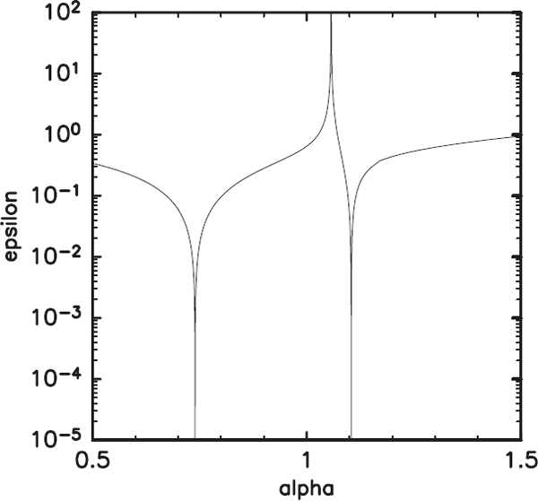
We repeat the integration with changing α continuously in the range of 0.5 ≤ α ≤ 1.5 and evaluate the left-hand side of (18). Figure 2 presents the dependence of ε = |(X − ̃HY)/X| (ζ = 0) on α. Similar to that shown by Salby (1979), there are two distinct dips, but at α = 0.739 and α = 1.107. The corresponding equivalent depths are h = 9.90 km and h = 6.61 km, respectively. In particular, the equivalent depth corresponding to the latter Pekeris mode is significantly different from the value obtained by Salby (1979). The possible reason for this is that the equivalent depth of the Pekeris mode strongly depends on the vertical temperature profile of the atmosphere and is strongly affected by the calculation errors that cannot be avoided in Salby's (1979) calculation method.

The vertical profiles of the disturbance amplitudes, |̃Z|, of the two modes obtained from the numerical calculations in this subsection are presented in Fig. 3. Note that the shown “amplitude” is the transformed one, |̃Z|, not |Z|. Similar to that shown by Salby (1979), the Pekeris mode (Fig. 3b) has a node in the stratosphere, whereas the amplitude of the Lamb mode (Fig. 3a) decreases monotonically, almost exponentially, with altitude. Note that the node of the Pekeris mode is located at a geometric altitude of around 22.5 km in this calculation, which is lower than that obtained by Salby (1979), 3.5H ≈ 25.5 km, there. We deduce that this discrepancy is a reflection of the accuracy problem with Salby's (1979) calculation method.
3.2 Numerical results using the sophisticated method
Similar to the previous subsection, we integrate the simultaneous ordinary differential equations (37) and (38) for (W, V) in the decreasing direction of ζ up to ζ = 0 by using the classical 4th-order Runge-Kutta method with giving the starting point condition (44) or (45) and examine the value of the left-hand side of (39). Numerical settings are the same as those of the previous subsection, but here, we take the altitude dependence of the gravity acceleration g (ζ) and the mean molecular weight M (ζ) described in USSA76 (Fig. 4).


Figure 5 presents the dependence of ≈ = |(V + (α̂H − 1/2)W)/W| (ζ = 0) on α. Although the shape of the graph is different from that of the graph presented in Fig. 2 due to the difference in the solved equations, there again are two distinct dips but at α = 0.739 and α = 1.114. The corresponding equivalent depths are h = 9.90 km and h = 6.57 km, respectively. Whereas the equivalent depth of the former Lamb mode is the same as the value obtained in the previous subsection, the equivalent depth of the latter Pekeris mode is slightly smaller than the value obtained in the previous subsection. This difference is caused by the inclusion of the altitude dependence of the gravitational acceleration and the mean molecular weight. In fact, if the equations and boundary conditions used are left unchanged and the calculations are performed with these fixed at g0 and M0, the positions of the dips in the α − ε graph are exactly the same as in Fig. 2 (although the figure is not presented).

The vertical profiles of the disturbance amplitudes, |W|, of the two modes obtained from the numerical calculations in this subsection are presented in Fig. 6. Note that the shown “amplitude” here is |W|, not |̃Z|. Displaying this quantity does not change the fact that the amplitude of the Lamb mode (Fig. 6a) decreases monotonically with altitude, but for the Pekeris mode (Fig. 6b), the node is at a geometric altitude of about 10.3 km. In the study by Watanabe et al. (2022), it was shown that the Pekeris mode simulated by a GCM (= General Circulation Model) had a node at a pressure level of about 90 hPa [c.f. Watanabe et al. (2022)'s Fig. 8b] with the amplitude being expressed in terms of vertical p-velocity (ω). Here, note that ω ∝ −e−̂z/(2H)W, and the node of ω should be compared with that of W. Because the pressure level of 90 hPa is at a geometric altitude of about 17 km in USSA76, the altitude of the node of the Pekeris mode determined by Watanabe et al. (2022) is considerably higher than that determined in this subsection. This discrepancy could be due to differences in the vertical profiles of background temperatures or to some imperfection in the GCM used in the study by Watanabe et al. (2022).

Because the drawn profiles are for |W| in Fig. 6, which does not correspond to |Z| shown in Fig. 3, we cannot compare these profiles directly. Instead of |W|, Fig. 7 draws the profiles of |UH| for U defined by (46). Comparing Figs. 3 and 7, it can be seen that although the solution methods are different, the obtained amplitude profiles of the eigenfunctions are almost identical except for constant multiples. Note also that it is natural that the altitudes of the nodes are displaced between |W| presented in Fig. 6b and |UH| presented in Fig. 7b, considering the continuity equation because U corresponds to the horizontal convergence.

The results shown in Figs. 2 and 5 are based on the geometrical altitude of the upper boundary of 1000 km, but Salby (1979) seems to set the geometrical altitude of the upper boundary to 60H ≈ 440 km. Therefore, we have done the same computations except for setting the upper boundary to 440 km, the α − ε graph hardly changes (not shown), and the equivalent depths of the Lamb and Pekeris modes are not changed with an accuracy of three significant digits.
Depending on the setting of the position of the top boundary, however, perfect resonance may occur and the value of the equivalent depth may be slightly shifted. Figure 8 presents the α − ε graph for the case where the upper boundary is set to be 91 km (the upper edge of the lowest temperature region in USSA76). In this case, the positions of the dips are at α = 0.739 and α = 1.104, where ? goes to zero. This means that a perfect resonance occurs, and the Lamb and Pekeris modes are exactly free oscillation modes. The reason for this perfect resonance is that the atmospheric temperature is low at 91 km, where r < 0, and evanescent solutions are selected. In this case, the equivalent depth of the Lamb mode remains unchanged at 9.90 km, whereas that of the Pekeris mode is 6.63 km.
From the results shown above, as long as the vertical temperature profile defined as USSA76 is used, we can conclude that the equivalent depths of the Lamb and Pekeris modes are 9.9 km and 6.6 km, respectively, with an accuracy of two significant digits if the upper boundary for the computation is above the lower edge of the thermosphere. In the present manuscript, the altitude dependence of the gravity acceleration and the mean molecular weight are considered. In the thermosphere, the specific heat ratio γ should also change with height, but this is not taken into account (in USSA76, only the information that γ = 1.4 is given, and the altitude dependence of γ is not described). However, considering the fact that the equivalent depths of the Lamb and the Pekeris modes did not change between the above calculations with setting the upper boundary to 1000 km and that with setting the upper boundary to 440 km (even though the mean molecular weight is nearly five times different at those two altitudes), it is considered that even if the dependence of γ on the altitude is given accurately, it will not affect the calculation of equivalent depth.
4. Summary and discussion
In the present manuscript, we re-examined the calculation of Salby (1979) in relation to the Pekeris mode, which was firstly detected by Watanabe et al. (2022) from observations of waves generated by the eruption of Tonga, so as to examine what its equivalent depth value would be under a standard vertical atmospheric temperature profile such as USSA76. After examining the calculation of Salby (1979), it was found that the transformation of the equation there was inappropriate for the case where there is a discontinuity in the vertical temperature gradient, such as USSA76. Therefore, in the present manuscript, we presented an improved calculation method and calculated the equivalent depths for the Lamb and Pekeris modes. In addition, several calculations were performed for different position settings for the upper boundary, considering the altitude dependence of the gravity acceleration and mean molecular weight, which were not taken into consideration by Salby (1979). It is concluded that the equivalent depth values obtained by Salby (1979) are incorrect, and that under the atmospheric temperature profile of USSA76, the equivalent depths of the Lamb and Pekeris modes are 9.9 km and 6.6 km, respectively, in two significant digits (The equivalent depth of the Pekeris mode slightly varies depending on the setting of the position of the upper boundary, but does not change within the range of two significant digits).
The equivalent depth of 6.6 km for the Pekeris mode obtained in the present manuscript is larger than that of 6.1 km estimated from the observation of waves generated by the eruption of Tonga in the study by Watanabe et al. (2022). There seems to be two main reasons for this discrepancy. First, the USSA76 vertical temperature profile used in the present manuscript is for midlatitudes, which may be different from the vertical temperature profile at the latitudes where the Pekeris mode was excited and where it propagated by the time used to determine its phase velocity. Second, Watanabe et al. (2022) estimated the phase velocity of waves from observations: it is possible that the phase velocity can differ from that of the stationary atmosphere due to background winds. We should also note here that in the study by Watanabe et al. (2022), they also conducted a spectral analysis of 57 years of hourly global reanalysis data and demonstrated that there was a distinct spectral peak corresponding to the Pekeris mode [Watanabe et al. (2022)'s Fig. 9d], but the corresponding equivalent depth for the spectral peak seemed to be larger than 6.1 km. This may imply that the long-term climatological value of the equivalent depth of the Pekeris mode may be close to the value determined in the present manuscript, 6.6 km. To determine which of the aforementioned reasons may be responsible for the discrepancy between the equivalent depth of the Pekeris mode obtained in the present manuscript and that estimated by Watanabe et al. (2022), the first step would be to calculate the equivalent depth using the present method, given the horizontally averaged vertical temperature profile of the atmosphere at the time of Tonga's eruption, which will be our next work.
Supplements
Supplement 1 is a Fortran90 program that computes the α dependence of ε shown in the present manuscript. The terms and conditions of the program are subject to the JMSJ Submission Regulation.
Data Availability Statement
All data analyzed in this study are generated by the supplement program.
Acknowledgments
We thank Dr. Takatoshi Sakazaki, two anonymous reviewers, and the journal editors for their helpful comments. Special thanks to one of the reviewers for pointing out a serious error in the original version of the manuscript. This work was supported by JSPS KAKENHI Grant Numbers 20K04061.
The GFD-DENNOU Library (https://www.gfddennou.org/arch/dcl/) was used to draw the figures.
References
- Andrews, D. G., J. R. Holton, and C. B. Leovy, 1987: Middle Atmosphere Dynamics. Academic Press, 489 pp.
- Gill, A. E., 1982: Atmosphere-Ocean Dynamics. Academic Press, 680 pp.
- NOAA, NASA, and USAF, 1976: U.S. Standard Atmosphere, 1976. U.S. Government Printing Office, 227 pp.
- Pekeris, C. L., 1937: Atmospheric oscillations. Proceedings of the Royal Society of London, A158, 650-671.
- Sakazaki, T., and K. Hamilton, 2020: An array of ringing global free modes discovered in tropical surface pressure data. J. Atmos. Sci., 77, 2519-2539.
- Salby, M. L., 1979: On the solution of the homogeneous vertical structure problem for long-period oscillations. J. Atmos. Sci., 36, 2350-2359.
- Watanabe, S., K. Hamilton, T. Sakazaki, and M. Nakano, 2022: First detection of the Pekeris internal global atmospheric resonance: Evidence from the 2022 Tonga erupand from global reanalysis data. J. Atmos. Sci., 79, 3027-3043.