Development and validation of the SPEC model for simulating the fate and transport of pesticide applied to Japanese upland agricultural soil

Abstract

A pesticide fate and transport model, SPEC, was developed for assessing Soil-PEC (Predicted Environmental Concentrations in agricultural soils) for pesticide residues in upland field environments. The SPEC model was validated for predicting the water content and concentrations of atrazine and metolachlor in 5-cm deep soil. Uncertainty and sensitivity analyses were used to evaluate the robustness of the model’s predictions. The predicted daily soil water contents were accurate regarding the number of observation points (n=269). The coefficient of determination (R²) and Nash-Sutcliffe efficiency (N_SE) were equal to 0.38 and 0.22, respectively. The predicted daily concentrations of atrazine and metolachlor were also satisfactory since the R² and N_SE statistics were greater than 0.91 and 0.76, respectively. The field capacity, the saturated water content of the soil and the Q₁₀ parameter were identified as major contributors to variation in predicted soil water content or/and herbicide concentrations.

Introduction

Pesticides have been commonly used in agriculture since the second half of the twentieth century.^1,2) The widespread use of pesticides, however, has resulted in drift, leaching, and the runoff of pesticide from target crops to off-target areas which can aversively impact the environment.²⁾ Indeed, agriculture has been reported as the main source of groundwater contamination and numerous monitoring studies have highlighted the presence of pesticides in agricultural soils and surface and ground bodies of water.^3–5) In Japan, the persistence of pesticides in agricultural soils is evaluated in accordance with the test guidelines prescribed by the Ministry of Agriculture, Forestry and Fisheries⁶⁾ in limited conditions or simple scenarios. Meanwhile, the Ministry of Health, Labor and Welfare announced new standards for Maximum Residue Limits (MRLs) for pesticides in food and food additives (Positive List System) in 2003.⁷⁾ In the so-called Positive List System, MRLs of 0.01 ppm were assigned for all of the registered combinations of crops and pesticides that had been previously neglected. These low MRLs have raised concerns about the increased probability of exceeding the MRLs in crops. Indeed, in agricultural fields where crop rotation is used, the residues of pesticides applied to the previous crop may be taken up by the next crop depending on the persistence and uptake characteristics.

To conduct realistic assessments of pesticide residues in soil for the purpose of adapting to the new regulations, a model simulation could be one practical alternative to pesticide monitoring and experiments that are often expensive and time consuming. By taking into account the major processes involved in the environmental fate of pesticides (sorption, degradation, leaching, volatilization, and runoff), models can be used for pesticide registration, mitigation, risk assessment, and screening purposes.^8–10) Modeling approaches vary in complexity and can be classified as deterministic or stochastic models with two subcategories, mechanistic and functional.¹¹⁾ Models based on simple lumped parameters are limited to the relative ranking of hazardous chemicals but have the potential to be used for preliminary risk assessment. In contrast, models based on distributed parameters are more comprehensive in the level of detail and can account for the heterogeneity of the environment. In practice, however their use is limited due to impractical data requirements.²⁾

In Japan, the development of pesticide models for investigating the fate and transport of pesticides applied to lowland rice paddy fields has been reported.^12–17) However there is not yet a pesticide fate and transport model that simulates the behavior of pesticides applied to Japanese upland agricultural soil. This could be due to the necessity of validating models through testing against high-quality field data sets.⁹⁾ The aim of this research was thus: (1) to develop a pesticide fate and transport model, the SPEC model, (2) to evaluate the predictions of the model using field monitoring data and, and (3) to conduct uncertainty and sensitivity analyses of the SPEC model.

Materials and Methods

1. Model description

The SPEC model was designed to assess the Soil-PEC (Predicted Environmental Concentrations in agricultural soils) of pesticides. The model, coded in Visual Basic for Application in MS Excel, is a lumped parameter, one-dimensional, field scale, and daily time-scale model. The properties of the soil layers are assumed to be homogeneous; a maximum of two soil layers can be defined in the model while a maximum of three successive applications of pesticide can be scheduled. The depth of the soil layers is defined by the user. Groundwater flow or recharge is not considered in the model. Then, the soil water content and pesticide concentrations are calculated successively, from top to bottom. The SPEC model does not simulate the subsurface lateral flow, macropore flow, bypass flow, or tile drainage. Fig. 1 shows the current conceptual SPEC model and the various hydrological and pesticide fate and transport processes considered by the model. The SPEC model estimates water runoff, leaching, and associated pesticide loading. The Soil Conservation Service (SCS) curve number technique developed by the USDS is used to estimate runoff whereas infiltration is determined by using a storage routing methodology. Such a scheme is often referred to as “tipping bucket” in the literature.¹⁸⁾ As compared with other pollutant fate and transport fate models (PRZM, HYDRUS, MACRO), SPEC development focuses on having minimum input parameter requirements while maintaining physically based processes. The mass balance equation used by the SPEC model to calculate the amount of water in the soil layers is:   

(1)

  

(2)

where the subscripts i and j specify the day and the soil layer of the variables. To clearly display the processes that are considered in soil layers 1 and 2 in Eq. (1), the subscript j was explicitly replaced by the soil layer number (1 or 2). WC_i+1,j and WC_i,j are the water contents expressed as water depths (using Eq. (2)) for day i+1 and i of the soil layer j (mm), respectively; Rain_i is the amount of rainfall that occurred during day i (mm), INF_i,1 and INF_i,2 are the amount of infiltration on day i from soil layers 1 and 2 (mm), respectively; ET_i,1 and ET_i,2 are the amounts of water removed from soil layers 1 and 2 (mm) due to evapotranspiration; depth_j is the depth of the soil layer j (cm); ρ_b is the bulk density of the soil (g cm⁻³); and θ_i,j is the volumetric water content of soil layer j for day i (cm³/cm³). The methodology implemented to calculate each process is detailed in the next section while the processes considered to simulate pesticide fate and transport including pesticide loss through percolation, runoff, and biochemical and photochemical degradations are presented in Section 3.

Fig. 1. Conceptual hydrological and pesticide fate and transport processes considered by the SPEC model in a bare soil, upland field. Plain arrows represent the hydrological processes while dashed arrows characterize the pesticide fate and transport processes.

2. Field-scale hydrological processes

2.1. Infiltration

The daily infiltration of water is related to the current water content of the soil and the soil’s ability to hold water. Water infiltrates from a soil layer to the soil layer below if the water content of the soil layer exceeds the field capacity of that layer and the layer below is not saturated. The amount of water available for infiltration in a soil layer is therefore given by:   

(3)

where WCX_i,j is the drainable volume of water through infiltration in soil layer j on day i (mm), and WC_i,j and FC_j are the water content and field capacity at iteration i of soil layer j (mm), respectively. Next, the amount of water that actually moves from one soil layer to the soil layer below is calculated the storage routing methodology¹⁹⁾:   

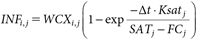(4)

where INF_i,j is the amount of water that infiltrates from soil layer j to the underlying soil layer at iteration i (mm), Δt is the length of the time step (h), Ksat_j is the saturated hydraulic conductivity for layer j (mm/h), SAT_j is the saturated water content of layer j (cm³/cm³), and the other parameters are as previously defined.

2.2. Surface runoff

Pesticide losses through surface runoff depend on the amounts of available pesticides in the soil surface, their chemical properties, and the intensities of rainfall and runoff.²⁰⁾ In the SPEC model, surface runoff is only computed for the topsoil layer, using the SCS curve number procedure. The SCS curve method is an empirical method developed through more than 20 years of studies involving rainfall-runoff relationships across the USA.²¹⁾ The method was developed to take into account different categories of land use and soil type. While the SCS curve method was reported to be appropriate for Japanese soil conditions on a watershed scale, there have been few reports regarding its application on a field scale.²²⁾ The SCS curve number equation is defined as²³⁾:   

(5)

where Runoff_i,1 is the runoff amount generated at time i by the topsoil layer (mm), S_i is the retention parameter of the soil on day i (mm), and I_a is the initial abstraction which includes surface storage, interception and infiltration prior to runoff (mm). For runoff to occur, the condition Rain_i>I_a must be met. In the SPEC model, I_a was approximated as 0.2S as it is commonly reported in the literature.¹⁹⁾ The curve number of the soil is related to the retention parameter of the soil S_i, as illustrated in Eq. (6):   

(6)

where CN_i is the curve number for day i of the top soil layer (dimensionless). Three moisture conditions are defined in the SCS curve number method: dry (CN1), average (CN2), and wet (CN3). CN2 is required as a parameter input; an appropriate value can be extracted from the literature for various combinations of land use and soil type.^19,23) Note that these CN values are recommended for a 5% slope; if the slope of the field is different, the CN number must be adjusted.   

(7)

where CN2_adjust is the CN2 value adjusted for slope and slp is the average slope of the field (%). CN1 and CN3 are respectively the lowest and highest boundaries of the CN value. They are evaluated once, at the beginning of the simulation, using Eqs. (8) and (9):   

(8)

  

(9)

CN1 and CN3 remain constant during the whole simulation and can be seen as properties of the soil. The retention parameter (S_i) varies depending on the daily moisture of the soil and is re-evaluated at each computation iteration using the following equation:   

(10)

where S_i is the retention parameter at time i (mm), S_max is the maximum value the retention parameter can achieve on any given day (mm), WC_i is the soil water content of the soil layer (mm), W_res is the water residue of the soil layer (mm), and w₁ and w₂ are shape coefficients. S_max can be calculated from Eq. (5) by replacing CN_i with CN1. Once the retention parameter of the soil for the day is known, the value of the daily curve number can be calculated by rearranging Eq. (6):   

(11)

where CN_i and S_i are the curve number and the retention parameter for day i (mm), respectively. In practice, the method is implemented as follows: first, the CN1 and CN3 of the soil are computed (Eqs. (8) and (9)). Then, every computation iteration, S, is calculated using Eq. (10), and the amount of runoff is evaluated using Eq. (5).

An option to cancel runoff has been implemented in the model. Indeed, during field experiments conducted to validate the model, borders were installed between fields to avoid the potential cross-contamination of pesticides. As a result the surface runoff of each plot was confined within that plot.²⁴⁾ When the “no-runoff” option is used, water that was supposed to be lost due to water runoff is routed to infiltration therefore increasing the amount of infiltrating water. Note that, in the case of irrigation, the amount of irrigation water was added to the amount of precipitation as input water.

2.3. Evapotranspiration

Two options have been implemented in the SPEC model regarding evapotranspiration (ET). The first option is used when no data are available. A constant daily value is used throughout the simulation. The second option uses the Penman-Monteith equation to predict daily evapotranspiration (ET_c). The procedure for calculating all variables can be found in Allen et al.²⁵⁾

Since ET_c is computed by assuming that the plant had optimum soil water conditions, the actual evapotranspiration of the field must be adjusted to reflect current field conditions. The actual amount of water removed from the two soil layers by evapotranspiration is proportional to the depth of the soil layers and is calculated using Eq. (12):   

(12)

where ET_i,1 and ET_i,2 are the actual evapotranspiration losses at day i from soil layers 1 and 2 (mm), respectively, WC_i,1 and WC_i,2 are the amounts of water held in soil layers 1 and 2 (mm), respectively, FC is the soil field capacity (mm) of the soil layer, and depth₁ and depth₂ are the depths of soil layers 1 and 2 (cm), respectively．

3. Pesticide fate and transport

Pesticide is introduced in the model by scheduling a pesticide application. The user is required to input the date and the rate pesticide application. Then, the fate and transport of the pesticide in the field are simulated by considering various pesticide degradations, loss of pesticide by surface runoff, and pesticide transport through vertical percolation in and out of the soil layers. Consequently, the equation used to predict pesticide concentrations in the two soil layers is:   

(13)

where Mp_i,1 and Mp_i,2 are the mass of pesticide in soil layers 1 and 2 at time i (mg), respectively, Mp_i−1,1 Mp_i−1,2 are the masses of pesticide in soil layer 1 and 2 at time i−1 (mg), respectively, Mrunoff_i,1 is the mass of pesticide lost through runoff from the topsoil layer at time i (mg), and Mperc_i,1 and Mperc_i,2 are the masses of pesticide lost through percolation at time i by soil layers 1 and 2 (mg), respectively. Mphoto_i,1, is the mass of pesticide loss through photodegradation in the topsoil layer at time i (mg), and Mbio_i,1, Mbio_i,2 and are the masses of pesticide loss trough biochemical degradation at time i (mg), in soil layers 1 and 2, respectively.

3.1. Pesticide transported by surface runoff

The mass of pesticide loss from the soil top layer through water runoff is calculated by:   

(14)

where Cs_j is the pesticide concentration in soil layer j (mg/kg), K_d is the soil adsorption coefficient of the pesticide in the soil (L/kg) and the other parameters are as previously defined. The soil adsorption coefficient of the pesticide in the soil is related to the soil organic content, Oc (%). The relation is given as:   

(15)

where K_oc is the soil organic-water partitioning coefficient of the pesticide (L/kg) and Oc is the percentage of soil organic carbon (%). Note that the transport of pesticide sorbed to soil particles with surface runoff is not considered in the current model.

3.2. Pesticide transport via vertical percolation

In the SPEC model, the amount of pesticide that is transported with percolating water is a function of infiltration:   

(16)

where Mperc_i,j is the mass of pesticide loss from soil layer j at iteration i (mg), INF_i,j is the amount of water that percolates from the layer j (mm), and all other variables are as previously defined. The mass of pesticide loss by percolation by soil layer j is added to the mass of pesticide in the soil layer j+1 (Eq. (13)).

3.3. Pesticide biochemical degradation

Pesticide biochemical degradation was describe by a first-order equation:   

(17)

where Mbio_i,j is the mass of pesticide loss from soil layer j at iteration i by biochemical degradation (mg), ρ_b is the bulk density of the soil (g/cm³), and k_bio is the first-order rate constant of the pesticide biochemical degradation in the soil (1/day). The first-order rate constant degradation is calculated from the half-life of the pesticide’s biochemical degradation:   

(18)

where HL_bio is the pesticide half-life of biochemical degradation (day).

The influence of temperature on the degradation rate can be accounted for in the temperature data as: (1) two average temperatures with their corresponding periods, (2) daily average temperatures, and (3) hourly average temperatures. Using the first option, two degradation rates are computed and used during the appropriate periods. In contrast, when using options 2 and 3, the degradation rate can change on a daily or hourly basis. The equation used to adjust the half-life of a pesticide due to temperature is given as²⁶⁾:   

(19)

where k_bioref is the reference pesticide’s half-life at 25°C (day), Q₁₀ is the change of half-life given a 10°C change in temperature (unitless), and t₁ is the temperature at which the half-life of the pesticide must be calculated (°C).

3.4. Photochemical degradation

Photodegradation was reported to be one of the most destructive pathways for pesticides after their release into the environment.²⁷⁾ This process in soil surfaces is only significant if there is no foliage covering the ground. In the SPEC model, this process is only considered in 2-mm depth of the topsoil layer. To accurately determine the loss of pesticide by photodegradation, the level of solar radiation reaching the ground must be known. This is evaluated using the following equation which was originally developed for paddy fields¹⁵⁾:   

(20)

where R_UVB-a and R_UVB-b are the daily UV-B radiation above and below the plant canopy (MJ/m²), respectively, f_R-ab is the slope of the fitted line obtained from the relative difference of the radiation above and below the plant canopy that accounts for the light attenuation by the growing crop, and t is the time (day). The UV-B radiation reaching the ground can be calculated as:   

(21)

where f_US is the fraction of the UV-B radiation over the solar radiation, and R_S-a is the solar radiation below the plant canopy. When no plants are growing in the field (bare soil condition), f_R-ab is equal to 0 and the UV-B radiation above and below the plant canopy is identical. The final equation used to compute the mass of pesticide loss by photodegradation is:   

(22)

where Mphoto_i,1 is the mass of pesticide loss by photodegradation (mg), k_photo is the first-order rate coefficient of photochemical degradation with respect to cumulative UV-B radiation (m²M/J), and all other parameters are as previously defined. The first-order rate coefficient of photochemical degradation with respect to cumulative UV-B radiation can be calculated from the half-life of pesticide photodegradation.   

(23)

where HL_photo is the photochemical degradation half-life of the pesticide (day), and Solar is the average solar radiation measured during the experiment duration (MJ/m²/day). While determining k_photo experimentally at a site is preferable for accurately predicting the photodegradation of pesticides, Eq. (22) can be used to derive k_photo from existing pesticide databases.

4. Field experiments

We attempted to validate the SPEC model so as to predict: (1) soil water content and (2) the concentrations of two herbicides: atrazine and metolachlor. All observed data were acquired over a two-year monitoring period (2013–2014) at the experimental farm of Tokyo University of Agriculture and Technology (TUAT experimental farm), Tokyo, Japan. Details of the experiment can be found elsewhere.²⁴⁾ Briefly, the field was divided into three experimental plots that were surrounded by plastic borders buried approximately 10 cm in the ground. Note that the borders prevented surface runoff from the plots. The texture of the soil was identified as clay-loam while its taxonomic order is andisol. It contained 29.6% sand, 33.4% silt, and 23.4% clay. Some characteristics of the soil are reported in Table 1. Atrazine and metolachlor were applied twice, on June 10, 2013 and December 6, 2013 to the whole surface of the plots. The commercial formulation of the herbicides (Geza non gold^® Syngenta, Tokyo, Japan) was diluted with distilled water and applied at the recommended rates of 771.3 and 732 g a.i./ha for atrazine and metolachlor, respectively. Neither herbicide was applied to the field prior to the experiment and no crops were grown on the plots. In addition, no irrigation water was applied to the field during the entire duration of the experiment.²⁴⁾ Precipitation, soil temperature, and soil moisture contents at 5.0 cm deep were recorded hourly.²⁴⁾ Soil samples were collected at a depth of 5 cm at specified intervals from the three plots using soil cores 5 cm in diameter. A composite sample was created for each plot by mixing three samples taken randomly from each plot. The procedure used to clean up the composite samples and extract the pesticide can be found in the literature.²³⁾

Table 1. List of the input parameters used to simulate the soil water content and the concentrations of atrazine and metolachlor in TUAT experimental farm

SPEC model inputs	Abbreviations	Units	Atrazine	Metolachlor
Field
Organic carbon	Oc	%	6.9524)
Bulk density	ρb	g/cm	0.524)
Saturated water content	SAT	cm3/cm	0.9524)
Water residue	Wres	cm3/cm	0.10a
Saturated hydraulic conductivity	Ksat	Cm/h	10.80a
Curve number	CN	—	8623)
Slope	slp	%	524)
Field capacity	FC	cm3/cm	0.4024)
Pesticide
Date of applications	—	Date	10 June 2013, 6 December 2013
Application rate	—	g/ha	771.324)	732.524)
Partitioning water organic coefficient	Kd	L/kg	10028)	12024)
Half-life biochemical degradation	HLbio	day	23.528)	24.728)
Half-life photo-degradation	HLphoto	day	10029)	199a
Average solar radiation	Solar	kJ/m	1424)	14a
Q10	Q10	—	1.3524)	1.4224)

Note: ^a Input was calibrated.

5. Model parameterization

The input parameters used for predicting soil moisture and concentrations of atrazine and metolachlor at the TUAT experimental farm are reported in Table 1. Soil layers 1 and 2 were 1 cm and 4 cm deep, respectively. The data used to parameterize the model were taken from the literature or database. When no data were available, the inputs were calibrated.^21,24,28,29) The curve number value used in the simulation was extracted from the tables provided by the SCS Engineering Division and is appropriate for a 5% slope with bare soil (no crop residue) and a soil with moderate infiltration rate.¹⁹⁾ Previous analysis indicated that the curve number method was applicable for the andisol soil plot scale with bare soil. The method was, however, sensitive regarding the initial moisture content of the soil.³⁰⁾ Nevertheless, further validation of the method of application in Japan for other combinations of land cover and soil conditions is necessary. Hourly monitored precipitation and temperature data were used for the simulation. Daily average solar radiation as well as minimum, maximum, and average daily air temperature data was downloaded from the AMEDAS weather station located about 500 m from the monitoring site in Fuchu City, Tokyo (Japan).³¹⁾ These data were used to calculate the daily amount of evapotranspiration from the TUAT experimental farm.²⁵⁾

6. Sensitivity and uncertainty analyses

The possible application of any model and its validation procedures are largely determined by the model’s sensitivity.¹¹⁾ Indeed, input parameters are variable which can be attributed to (1) protocols and analytical methods and (2) spatial variability that occurs naturally.¹¹⁾ Since input parameters must be estimated whenever data are missing, characterizing and ranking input parameters as to their influence on model predictions are absolutely necessary to correctly interpret a models’ output. Uncertainty and sensitivity analyses were performed by applying Monte Carlo (MC) techniques to the SPEC model. To noticeably recognize the effects of uncertainty included in input parameters on the predicted soil water content and pesticide concentrations, two MC scenarios were created. The first MC scenario (MC scenario 1) included only input parameters related to soil properties while the second MC scenario (MC scenario 2) consisted of input parameters related to pesticide characteristics.

The water residue (W_res), the saturated hydraulic conductivity (K_Sat), the saturated water content (SAT_j) and the field capacity (FC_j) of the soil were included in the first MC scenario for a total of four investigated input parameters. Three parameters were considered in the second MC scenario: the photodegradation half-life (HL_photo), the Q₁₀, and the soil organic-water partitioning coefficient of the pesticide (K_oc). To avoid redundancy, the k_bio was not included in the analysis, since it is nested with the Q₁₀ parameter (Eq. (18)). In addition, accurate k_bio data from laboratory experiments (unpublished data, Table 1) were available for both atrazine and metolachlor. The sample size used for the MC simulations was 250 for both soil and pesticide parameter scenarios. This sample size proved sufficient for a pesticide fate and transport model in the case of pesticide applied in rice paddies.³²⁾ Uniform distributions were given to all investigated parameters. All parameters except the Q₁₀ parameter were allowed to vary a maximum of ±10% from the values used in the deterministic scenario presented in Table 1. The range of the Q₁₀ parameter was 1.0 to 2.2. A value of 1.0 indicates that temperature has no effect on the degradation half-life. A value of 2.2 was recommended for use when no site data was available.²⁶⁾ Note that the maximum range of the saturated water content of the soil was to 1.0 as values higher than 1.0 are not physically possible. For evaluating model response the soil water content and herbicide concentrations, target outputs were selected 24 days after the herbicide applications. This corresponds to the half-life period of appreciable herbicide concentrations; therefore the data set is representative of each season.

To visualize the evolution of output uncertainty every computation step, the 95th percentiles of the predicted soil water content and herbicide concentrations were plotted together with the predictions of the deterministic scenario.

The method used to measure input sensitivity was reported previously.^32,33) The method relies on a stepwise regression analysis that computes standard rank regression coefficients (SRRCs) for the predictors (inputs) that have the most significant influence on the predictions (outputs). By ranking the input parameters by absolute values of SRRCs, the model’s most sensitive parameters can be highlighted.

7. Model evaluation

The model’s accuracy regarding the predictions of soil water content and herbicide concentrations was evaluated using statistical indices. The coefficient of determination (R²) which describes the degree of collinearity between the simulated and measured data was reported to be extremely sensitive to extremely high values (outliers) and insensitive to additive and proportional differences between model predictions and measured data.³⁴⁾ Therefore to appropriately interpret the accuracy of a model, it is necessary to report additional statistical indices such as the Nash-Sutcliffe efficiency (N_SE). N_SE is a normalized statistic that compares the measured data variance to the relative magnitude of the residual variance.³⁵⁾ N_SE statistic range between −∞ and 1.0, the latter being the optimal value. Positive values are generally viewed as acceptable levels of performance. In contrast, negative values indicate that the mean of the observed value is a better predictor than is the simulated value.³⁶⁾

The root mean square error (RMSE) is an error statistic because it indicates error in the units of the variable of interest (cm³/cm³ for the soil water content and mg/L for herbicide concentrations).³⁶⁾ A value of 0 indicates a perfect fit. Having an RMSE value of less than half the standard deviation of the measured data was reported to be appropriate.³⁷⁾ The coefficient of residual mass (CRM) indicates if the model overestimate or underestimate the observations, a perfect fit is indicated by a value of 0. Positive values indicate that the model has a tendency to underestimate the data while negative values indicate that the model tends to overestimate the observations.³⁸⁾ The equations used to compute the different indices have been commonly reported in the literature.^36,38)

Results and Discussion

1. Model validation for the prediction of soil water content

During field monitoring, the daily volumetric average of the soil water content varied from 0.34 to 0.40 cm³/cm³ during the summer and winter seasons, respectively.²⁴⁾ There is a clear correlation between precipitation and increased the soil water content (Fig. 2). In major precipitation events, soil water content increased sharply, since runoff amounts were rerouted to the percolation component, as indicated previously. In the field, no sign of ponding was observed during these intense precipitation events, indicating that significant runoff was unlikely to have occurred. However, the validation of runoff and the corresponding pesticide discharge components of the SPEC model is required. In general, the SPEC model accurately predicted the soil water content of the TUAT experimental farm for the duration of monitoring (Fig. 2). The sensor used to record the soil water content failed starting on the March 5, 2014 (Fig. 2). Consequently, the evaluation of the model is based on recording prior to the sensor’s failure.

Fig. 2. Predicted and observed daily water content in 5-cm deep soil at TUAT experimental farm from 10 June 2013 to 5 May 2014. The grey band indicates the 95th percentile confidence interval of the predicted soil water content acquire from the MC simulation 1.

Two scenarios were used to simulate the soil water content. In the first scenario, a constant value for ET (0.1 cm/day) was used during the entire simulation period (dotted line in Fig. 2). In contrast, for the second scenario, daily ETs computed by the Penman-Monteith algorithm were used in the model (solid line in Fig. 2). The effect of ET on the simulated soil water content was particularly clear during the winter season (Fig. 2). Indeed, the default ET value (0.1 cm/day) seems to be too high during the winter season (dotted line in Fig. 2). The average ETs calculated using the Penman–Monteith method were 0.1 and 0.06 cm/day for the summer and winter seasons, respectively. As a result, too much water is removed from the soil, which results in the underestimation of soil water content during this period. In contrast, using daily ET values greatly improved the accuracy of the simulations of soil water content.

The statistical evaluations of the SPEC model for the two scenarios are reported in Table 2. The CRM statistic indicates that the model has a slight tendency to overestimate the soil water content. The N_SE, and RMSE statistics were similar for the two scenarios using constant and daily ET values. In contrast, the R² value increased significantly for the simulation using daily ET values. Indeed, the high linear relationship between the predicted and observed soil water content can be observed graphically in Fig. 2. While the predicted daily soil water content values did not always match the observed values, the general trend of the observations is very well captured by the model’s simulation. In general, regarding the number of observation points (n=269), the temporal and spatial variations of the observed water contents and the daily predictions for both scenarios were classified as good.

Table 2. Statistical evaluation of the SPEC model regarding the prediction of soil water content, atrazine and metolachlor concentrations

Outputs	Water content		Atrazine		Metolachlor
Evapotranspiration	Const. ET	Daily ETs	Const. ET	Daily ETs	Const. ET	Daily ETs
R2	0.16	0.34	0.93	0.92	0.91	0.93
NSE	−3.88	−1.06	0.91	0.89	0.82	0.76
RMSE	0.09	0.05	0.41	0.45	0.53	0.61
CRM	0.09	−0.003	0.12	0.07	−0.21	−0.27

2. Model validation for the prediction of atrazine and metolachlor concentrations

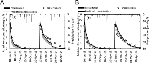
Atrazine and metolachlor concentrations were simulated from June 10, 2013 to May 5, 2014, using the input parameter values reported in Table 1 and the scenarios for constant and daily ET values. The deterministic simulations using the daily ET values are reported in Fig. 3 while the statistical evaluations of the model for both scenarios are reported in Table 2. The predicted herbicide concentrations for the two ET scenarios were similar, since the statistical evaluations of the two scenarios yield similar statistics for atrazine and metolachlor (Table 2). The model was flagged by the CRM statistics as slightly underestimating atrazine concentrations and overestimating metolachlor concentrations. Those trends were also confirmed by a visual inspection of the deterministic simulations of atrazine and metolachlor (Fig. 3). Nevertheless, the predicted herbicide concentrations are in range of the observations. Moreover, the N_SE was positive for all scenarios while the R² was higher than 0.90 for all scenarios. Thus, the model accurately simulated atrazine and metolachlor concentrations on the TUAT experimental farm.

Fig. 3. Predicted and observed concentrations of atrazine (A) and metolachlor (B) in 5-cm deep soil for the 1st MC scenario (parameter related to soil properties). Grey bands indicate 95th percentile confidence interval.

The dissipation behavior of the two herbicides was different between the summer and winter seasons as reported by the herbicide mass balance (Table 3). At the end of the seasons, the amounts of atrazine and metolachlor remaining in the soil layers were small. More herbicide was transported with vertical percolation during the summer season due to frequent and abundant precipitation events as compared to the winter season (Fig. 3). Note that since surface runoff was prevented due to the installation of borders surrounding the plot, herbicide was only transported through vertical percolation (Eq. (1)). It was anticipated that more herbicide mass would be lost through degradation during the summer season due to the effect of temperature on degradation. However, the percentage of atrazine loss through biochemical degradation during the winter season was higher than that of the summer season. The percentages of metolachlor loss through biochemical degradation in the summer and winter seasons were identical (Table 3). In the winter, less atrazine was lost through percolation, resulting in more chemicals available for biochemical degradation during the winter as compared to in the summer (Fig. 3). The amounts of herbicides lost through photodegradation during the summer and winter seasons were similar.

Table 3. Percentage of atrazine and metolachlor dissipated by various processes as compared to herbicides applied mass for the summer and winter seasons

Processes	Unit	Atrazine		Metolachlor
		Summer	Winter	Summer	Winter
Biochemical degradation	%	39	49	57	57
Photo-degradation	%	3	5	5	7
Percolation	%	58	46	39	33
Runoff	%	0	0	0	0
Residual dissolved into soil-water	%	<0.1	<0.1	<0.1	0.1
Residual sorbed onto soil-particles	%	<0.1	0.2	<0.1	2

Note: Runoff simulation was disabled for this simulation.

On February 15, 2014, a 9.5-cm precipitation event caused a great drop in predicted herbicide concentrations due to its transport through percolation bellow soil 5 cm deep (Fig. 3). However, the monitored herbicide concentrations, while decreasing, did not drop suddenly as the simulation had suggested. A possible explanation is that the model does not consider the effect of snowfall and snowmelt that occur at that time of the year. It was observed that snow melted gradually in the field and therefore, the actual amount of water that the soil received during a snowfall event was probably less than indicated in the data recorded by the logger. Note that the slight decline of observed herbicide concentrations due to precipitation on December 27 is well simulated by the model suggesting that the model’s assumptions are appropriate when there is no snowfall.

3. Uncertainty analyses

The effects of input uncertainty on the predicted soil water content and herbicide concentrations were investigated using two MC scenarios which consisted of: (1) soil parameter inputs and (2) herbicide characteristic inputs. The effects of uncertainty in soil parameters on the predictions of soil water content are reported in Fig. 2. The thickness of the 95th percentile confidence interval was constant through the simulation period, indicating that the influence of parameters’ uncertainty did not vary during the summer and winter seasons.

The results of the uncertainty analysis for the prediction of herbicide concentrations in soil are displayed in Fig. 3A, B for MC scenario 1 and in Fig. 4A, B for MC scenario 2, respectively. The effects of the soil property uncertainties on herbicide concentrations were consistent in the summer and winter seasons, as the thickness of the 95th percentile confidence interval remained constant throughout the simulation period (Fig. 3A, B). The 95th percentile confidence interval computed for atrazine was greater than that for metolachlor. Since the K_oc of atrazine is lower than that of metolachlor (Table 1), atrazine was simulated to be transported easily through water percolation which was flagged as a main route for herbicide dissipation (Table 3).

Fig. 4. Predicted and observed concentrations of atrazine (A) and metolachlor (B) in 5-cm deep soil for the 2nd MC scenario (parameter related to pesticide characteristics). Grey bands indicate 95th percentile confidence interval.

The herbicide characteristic uncertainties did not affect the predicted herbicide concentrations during the summer season (Fig. 4). In contrast, the predicted herbicide concentrations in the winter season were greatly affected by the herbicide characteristic uncertainties, as indicated with the greater thickness of the 95th percentile confidence interval. The K_oc parameter is used to predict the amount of herbicide transported with surface runoff and vertical percolation (Eqs. (14)–(16)). The Q₁₀ parameter is used together with the soil temperature to adjust the half-life of the biochemical degradation of herbicides (Eqs. (17)–(19)). Both infiltration and temperature data were reported to be significantly different between summer and winter seasons at the TUAT experimental farm (Table 3).²⁴⁾ Therefore, the differences in the effects of uncertainty included in herbicides’ characteristics between the summer and winter seasons on the predicted herbicide concentrations are due to different combinations of the interrelated parameters of K_oc and infiltration (Eqs. (14)–(16)) or Q₁₀ and temperature (Eqs. (17)–(19)). This result also suggests that it is appropriate to investigate the sensitivity of input parameters separately for summer and winter datasets. Note that solar radiation data were similar for the summer and winter seasons, 13.6±6.6 and 12.9±6.8 MJ m⁻², respectively. Consequently, the effect of the HL_photo input’s uncertainty on herbicide concentrations is constant regardless of the season (Eq. (22)). In the SPEC model, the parameter f_US (Eq. (21)) was constant during the simulation period. However, in practice this parameter fluctuates; therefore photodegradation was likely overestimated during the winter season.

4. Sensitivity analyses

Prior to the sensitivity analysis, all data generated by the MC simulations was assessed and showed no evidence of skewness or kurtosis for any of the input parameters and outputs. Consequently, a stepwise regression analysis was performed using an SPSS software package for statistical analysis.³⁹⁾ There was no evidence that any of the input parameters exerted undue influence on the regression models. Moreover, no indication of multicollinearity (two or more highly correlated predictor variables) in the data was found. The standardized rank regression coefficients (SRRCs) obtained using stepwise regression methodology are presented in Tables 4 and 5 for MC scenario 1 and 2, respectively. SRRC values can vary from −1 to 1, and high absolute values of SRRCs indicate for sensitive parameters. A positive SRRC indicates that increasing the parameter value will increase the output considered, and vice versa.

Table 4. Standardized rank regression coefficients of the SPEC model parameters for the 1st MC scenario (parameter related to pesticide characteristics)

Outputs	Sensitive parameters	MC scenario 1
		Summer	Winter
Water content	FC	0.87	0.87
	SAT	0.30	0.30
Atrazine	FC	−0.60	−0.58
	SAT	0.47	0.48
Metolachlor	FC	−0.62	−0.63
	SAT	0.46	0.46

Table 5. Standardized rank regression coefficients of the SPEC model parameters for the 2nd MC scenario (parameter related to pesticide characteristics)

Outputs	Sensitive parameters	MC scenario 2
		Summer	Winter
Atrazine	HLphoto	0.78	—
	Q10	—	0.75
Metolachlor	HLphoto	0.55	—
	Q10	—	0.55

For MC scenario 1, the ranking of the sensitive parameters was consistent, regardless of the season (Table 4). While the “no-runoff” option is used, the field capacity (FC) and the saturated water content of the soil (SAT) were flagged as the most sensitive parameters regarding the prediction of soil water content. The SRRCs of these parameters were positive since increasing both parameters increases the predicted soil water content. Indeed, increasing the SAT and FC allows the soil to: (1) store more water, (2) retain more water in periods of no rainfall, and (3) generate less percolation (Eqs. (2) and (3)). The same parameters were retained by stepwise regression methodology that uses herbicide concentrations as outputs. The sign of the reported SRRCs helps to gain some insight into the model’s behavior. Increasing the field capacity of the soil decreases predicted herbicide concentrations. In contrast, increasing the saturated water content of the soil increases predicted concentrations of herbicide. The field capacity of the soil determines the amount of water that is available for infiltration (Eq. (2)) and consequently, increasing this parameter increases the loss of herbicide due to percolation. A field’s saturated water content is primarily used to determine the amount of percolating water (Eq. (3)). By setting a higher SAT_j value, the amount of percolating water will be reduced, thereby limiting the transport of herbicide.

MC scenario 2 also produced a consistent ranking of the sensitive parameter. However, the season affected the ranking of the parameters (Table 5). For the summer season, the photodegradation half-life was flagged as the most sensitive parameter. This result is caused by not including the biochemical degradation rate (k_bio) in the sensitivity analysis to avoid redundancy with the Q₁₀ parameter. In the summer, temperatures are close to the reference temperature of 25°C; consequently, the Q₁₀ parameter does not impact the rate of k_bio. The analysis of the mass balance of the two herbicides (Table 3), however revealed that the mass of herbicides lost through biochemical degradation is 8 to 10 times higher than that lost through photodegradation. Consequently, accurate k_bio parameters are absolutely crucial for accurately determining the fate and transport of atrazine and metolachlor in both summer and winter. Increasing the HL_photo slows the degradation of herbicide in the field, which results in higher herbicide concentrations in the soil. For the winter season, the Q₁₀ was highlighted as the most sensitive parameter. The Q₁₀ parameter is an indication as to what extent the half-life of a pesticide will deviate from its default value at 25°C when the temperature changes by ±10°C. Indeed, the Q₁₀ and k_bio are nested together (Eq. (18)), and the high sensitivity of the Q₁₀, therefore, implies that the k_bio has to be accurately determined to accurately predict herbicide concentrations (Table 3). In addition, there is limited information about Q₁₀ values for pesticide; this was reflected in the parameter’s rather wide range (1 to 2.2) which also contributed to the high overall sensitivity of the parameter (see Fig. 4 winter). During monitoring, the average temperature in the winter was 5±4°C.²⁴⁾ Since there is approximately a 20°C difference between the reference temperature of 25°C and the average temperature in winter, the half-life of the herbicides in winter was divided by the square of the Q₁₀ (Eq. (18)), resulting in much slower herbicide degradation. During the summer season, the temperatures were closer to the reference temperature and, thus, the Q₁₀ did not affect predicted herbicide concentrations.

Conclusion

The SPEC model was developed to assess Soil-PEC (Predicted Environmental Concentrations in agricultural soils). The model was then validated using a field experiment carried out from June 10, 2013, to May 5, 2014 in which the soil water content and concentrations of atrazine and metolachlor were monitored. The soil water content predicted were accurate regarding the time step, and R² and N_SE statistics were equal to 0.38 and 0.22, respectively. The predicted atrazine and metolachlor concentrations were also adequate, and the R² and N_SE statistics were higher than 0.91 and 0.76, respectively.

The performance of the model with uncertain inputs was investigated using the Monte Carlo technique. The model’s predictions were influenced constantly throughout the simulation period due to the uncertainty encompassed in soil properties. In contrast, only the predicted herbicide concentrations in the winter season were influenced by uncertainty arising from pesticide properties. While preventing surface runoff in the model, the field capacity and the saturated water content of the soil were identified as major contributors to variation in predicted soil water content and herbicide concentrations. In addition, the Q₁₀ parameter was also flagged as a major contributor to variation in predicted herbicide concentrations, especially during the winter season.

The SPEC model therefore, has the potential to accurately predict water content and pesticide concentrations in soil. Moreover, the detailed pesticide mass balance given by the model can be used to identify major dissipation pathways and evaluate the best options for improving environmental conditions associated with pesticide residues in agricultural soil. Future improvements include: (1) the validation of the runoff component that was disabled in this study, (2) the creation of multiple soil layers for the improved prediction of soil water content, and (3) the dynamic adjustment of UV-B radiation over solar radiation’s dependence on environmental factors for improving predictions of photodegradation.

Acknowledgment

This research was supported by the Environment Research and Technology Development Fund (4-1303). DQ Thuyet is a JSPS postdoctoral research fellow at the Graduate School of Agricultural and Life Science, The University of Tokyo.

References

• 1) A. Pivato, A. Barausse, F. Zecchinato, L. Palmeri, R. Raga, M. C. Lavagnolo and R. Cossu: Atmos. Environ. 111, 136–150 (2015).
• 2) M. M. Hantush, M. A. Mariño and M. R. Islam: J. Hydrol. (Amst.) 227, 66–83 (2000).
• 3) D. D. Giannouli and V. Z. Antonopoulos: J. Environ. Manage. 150, 508–515 (2015).
• 4) A. Hildebrandt, M. Guillamón, S. Lacorte, R. Tauler and D. Barceló: Water Res. 42, 3315–3326 (2008).
• 5) L. Guzzella, F. Pozzoni and G. Giuliano: Environ. Pollut. 142, 344–353 (2006).
• 6) Ministry of Agriculture: Forestry and Fisheries of Japan (MAFF): http://www.acis.famic.go.jp/shinsei/8147/8147.pdf (Accessed 1 Sep., 2016; in Japanese).
• 7) T. Nagayama: J. Pestic. Sci. 30, 418–425 (2005) (in Japanese).
• 8) J. M. Marín-Benito, V. Pot, L. Alletto, L. Mamy, C. Bedos, E. Barriuso and P. Benoit: Sci. Total Environ. 499, 533–545 (2014).
• 9) J. J. T. I. Boesten and B. Gottesbüren: Agric. Water Manage. 44, 283–305 (2000).
• 10) M. Trevisan, G. Errera, C. Vischetti and A. Walker: Agric. Water Manage. 44, 357–369 (2000).
• 11) R. Calvet: Eur. J. Agron. 4, 473–484 (1995).
• 12) H. Watanabe and K. Takagi: Environ. Technol. 21, 1379–1391 (2000).
• 13) H. Watanabe and K. Takagi: Environ. Technol. 21, 1393–1404 (2000).
• 14) J. Tournebize, H. Watanabe, K. Takagi and T. Nishimura: Paddy Water Environ. 4, 39–51 (2006).
• 15) H. Watanabe, K. Takagi and S. H. Vu: Pest Manag. Sci. 62, 20–29 (2006).
• 16) K. Inao and Y. Kitamura: Pestic. Sci. 55, 38–46 (1999).
• 17) N. Iwasaki, K. Inao, T. Iwafune, T. Horio and H. Obara: Limnology 13, 221–235 (2012).
• 18) M. Trevisan, G. Errera, G. Goerlitz, B. Remy and P. Sweeney: Agric. Water Manage. 44, 317–335 (2000).
• 19) S. L. Neitsch, J. G. Arnold, J. R. Kiniry and J. R. Willams: “Soil and water Assessment Tool, Theoretical Documentation, Version 2009” Texas Water Resources Institute, College Station, Temple, Texas, 2011.
• 20) K. Siimes, S. Rämö, L. Welling, U. Nikunen and P. Laitinen: Agric. Water Manage. 84, 53–64 (2006).
• 21) W. C. Boughton: Aust. J. Soil Res. 27, 511–523 (1989).
• 22) J. Boulange, H. Watanabe, K. Inao, T. Iwafune, M. Zhang, Y. Luo and J. Arnold: J. Hydrol. (Amst.) 517, 146–156 (2014).
• 23) USDA: “National Engineering Handbook, Section 4: Hydrology,” 1972.
• 24) P. Jaikaew, J. Boulange, D. Q. Thuyet, F. Malhat, S. Ishihara and H. Watanabe: Environ. Monit. Assess. 187, 760 (2015).
• 25) R. G. Allen, L. S. Pereira, D. Raes and M. Smith: “Crop evapotranspiration: Guidelines for computing crop water requirements. FAO Irrigation and Drainage Paper No. 56.” 1998.
• 26) Soil Modelling Workgroup (FOCUS): Soil persistence models and EU registration (1997) http://ec.europa.eu/food/plant/docs/pesticides_ppp_app-proc_guide_fate_soil-persistance-1997.pdf (Accessed 1 Sep., 2016).
• 27) T. Katagi: Rev. Environ. Contam. Toxicol. 182, 1–189 (2004).
• 28) K. A. Lewis, A. Green, J. Tzilivakis and D. Warner: The Pesticide Properties DataBase (PPDB),” Agriculture & Environment Research Unit (AERU), University of Hertfordshire, http://sitem.herts.ac.uk/aeru/ppdb/en/ (Accessed 1 Sep., 2016).
• 29) F. Xiaozhen, L. Bo and G. Aijun: J. Hazard. Mater. 117, 75–79 (2005).
• 30) F. Malhat: International SWAT-Asia Conference IV (SWAT-Asia IV), Tsukuba, (Ibaraki, Japan), 2015.
• 31) Japan Meteorological Agency: http://www.jma.go.jp/jma/index.html (Accessed 1 Sep., 2016).
• 32) J. Boulange, K. Kondo, T. K. Phong and H. Watanabe: J. Pestic. Sci. 37, 323–332 (2012).
• 33) K. Kondo, J. Boulange and W. Hirozumi: J. Pestic. Sci. 37, 312–322 (2012).
• 34) D. R. Legates and G. J. McCabe Jr.: Water Resour. Res. 35, 233–241 (1999).
• 35) J. E. Nash and J. V. Sutcliffe: J. Hydrol. (Amst.) 10, 282–290 (1970).
• 36) D. N. Moriasi, J. G. Arnold, M. W. Van Liew, R. L. Bingner, R. D. Harmel and T. L. Veith: Trans. ASABE 50, 885–900 (2007).
• 37) J. Singh, H. V. Knapp, J. G. Arnold and M. Demissie: J. Am. Water Resour. Assoc. 41, 343–360 (2005).
• 38) Y. Hosaini, M. Homaee, N. A. Karimian and S. Saadat: Int. J. Plant Prod. 3, 91–104 (2009).
• 39) IBM SPSS Statistics for Windows, Version 22.0, (Released 2013).