3. Numerical Analysis Method
The formation process of joint interface of MPW is reproduced by two 2D models based on the purposes and functionality of the simulation software. Model 1 (Emag-Mechanical model) using finite element method to reproduce the deformation behavior of flyer plate in the electromagnetic field.10) Model 2 (SPH model) using SPH method to reproduce metal jet emission and wavy interface formation process.11)
3.1 Model 1 (Emag-Mechanical model): Reproduction of the deformation behavior of flyer plate in the electromagnetic field
Model 1 is a coupled mechanical and electromagnetic fields model constructed in ANSYS Emag-Mechanical that reproduces the deformation behavior of the Al sheet in the electromagnetic field. This model is used to calculate the collision angle β between flyer plate and parent plate and the impact velocity of flyer plate v. Figure 4 shows the schematic diagram of Model 1. Model 1 consists of FEM circuit and FEM model. FEM circuit consists of inductance (L), capacitor (C) and resistance (R) and coil (2D metal conductor). FEM model consists of flyer plate, parent plate, coil, air, and infinite boundary. The coil in FEM circuit is coupled with the coil element in FEM model. The true stress-strain curves obtained at a high strain rate condition are selected as the constitutive models for reproducing the deformation behavior of metallic materials in the electromagnetic field.12) The properties of flyer plate, parent plate, coil and anvil are shown in Table 3.


Table 3 The properties of flyer plate, parent plate, coil and anvil used for Model 1.
In the Model 1, discharge current, magnetic flux and electromagnetic force were calculated by Emag. The deformation process of the flyer plate was calculated by Mechanical. Figure 5 shows the calculation cycle of β and v in Model 1. In one cycle of the calculation, the discharge current running through the coil was firstly calculated by FEM circuit in Emag. Secondly, by coupling the coil element, the discharge current was input into the FEM model in Emag to calculate the magnetic flux around the coil and the eddy current generated in the flyer plate. The electromagnetic force was calculated from the interaction between magnetic flux and eddy current in the flyer plate and then import into the FEM model in Mechanical. Thirdly, the deformation process of the flyer plate in the electromagnetic field was reproduced by FEM model in Mechanical. The geometry shape of flyer plate will be updated at the end of each cycle and reloaded for next cycle until the flyer plate collided with the parent plate. When flyer plate collides with parent plate, the angle between flyer plate and parent plate is defined as initial collision angle β0, the velocity of flyer plate is defined as initial impact velocity of flyer plate v0. β0 and v0 will be further import into Model 2 (SPH model) as initial conditions to reproduce the wavy interface formation process during the collision in MPW. The governing equations of electromagnetic field can be found in the previous report.10)

Model 2 is an analytical model that reproduces the collision process between metal plate and parent plate and the accompanying temperature rise using the SPH method. Figure 6 shows the schematic diagram of Model 2. This analytical model consists of flyer plate, parent plate and anvil. The symmetric system of Model 2 is a two-dimensional flat plate system assuming that the depth direction is infinite. The unit system was set to mm, mg, and ms. To reduce the computing elements, the space other than the flyer plate, parent plate and anvil was assumed as vacuum in this study. The dimensions of the flyer plate, parent plate and anvil in the analysis model are 3 mm long × 0.4 mm wide, 3.5 mm long × 0.3 mm wide and 4.5 mm long × 0.5 mm wide, respectively. The impact velocity of flyer plate v (it is referred to as impact velocity hereafter) and the collision angle β obtained from the analysis of Model 1 were set as the initial conditions for Model 2. A fixed layer was set as a boundary condition (v = 0) for SPH particles located at the top of Anvil. The parameters used in equation of state and constitutive model for flyer plate, parent plate and anvil are Al 1100-O, Steel 1006 and SS304 from ANSYS material library and listed in Table 4.


Table 4 The parameters used for equation of states and constitutive models for each material.
The smoothing length h of the SPH method is an important factor that significantly affects the accuracy of analysis results and analysis time. In this study, for the flyer plate and parent plate, the smoothing length of the area within 0.05 mm from the surface, where corresponds to the collision surface, was set as 1 µm to reproduce more detail of the collision behavior. The smoothing length of the region further away from the interface was divided into two parts and set as 2 µm and 4 µm to reduce the analysis time. The smoothing length of anvil was set as the largest of 10 µm due to no detailed collision behavior is needed to reproduce.
Gauge point is a function of AUTODYN, by installing a gauge point on a specific SPH particle, it is possible to know the time history change of the specific parameters (temperature, pressure, and specific internal energy, etc.) related to that particle. Each SPH particle can only be installed for one gauge point. In this study, we focused on the range 2.6∼2.9 mm away from the first impact point and installed 200 gauge points on the SPH particles at the collision surface region (0∼0.004 mm from metal surface) and each base metal (0.02 mm away from the metal surface) (as shown in Fig. 6).
4. Results and Discussion
4.1 Microstructure of the magnetic pulse welded Al/Fe joint interface
Figure 7 shows the SEM backscattered electron images of Al/Fe joint interface. Figure 7(b) and (c) show the enlarged image of white rectangle in Fig. 7(a). In Fig. 7(a), the left edge of the downside Al plate sharpened distinctly due to the dramatic deformation. This area is defined as the first impact area. Along the welding direction, the joint interface presents an inconstant characteristic. The interface morphology shows a trigger-like morphology with IML, as indicated by the gray area, located near the vicinity of interface area. Away from the first impact area, the joint interface firstly shows a fractured area with continuous IML adhered to the Fe surface, as shown in Fig. 7(b). It is considered that in this area, during the collision process, a weak bond is formed briefly and then broke. A sound bonding is usually cannot formed near the first impact area. Continuously, along the welding direction, the IML shows a gradually decreased tendency. Figure 7(c) shows the onset of the welding area. In this area, the IML at the interface becomes intermittent and thinner.

Figure 7(c) shows the high magnification FE-SEM image of the white dotted rectangle region in Fig. 7(b). The IML presents two different contrast areas: the brighter contrast zone is surrounded by Fe, and the darker contrast zone is located between the Fe and Al. The IML with bright contrast has a quite homogeneous structure, while the IML with darker contrast shows a heterogeneous structure and contains many Fe-rich fragments. The embedded Fe-rich fragments in IML may be firstly ejected out of the Fe surface by the intense impact force, and then wrapped into the local melted compound of Al and Fe by an intense shear force.13,14) Depending on the formation location and composition difference, the two kinds of IML were defined as Tail-side layer (TSL) and Front-side layer (FSL).6) TSL is formed at the rear of the wave region and enveloped by the Fe at the collision surface, while the FSL is formed at the front of the wave region and adjoined with the Al matrix.
4.2 Reproduction of electromagnetic field and calculation of collision angle and impact velocity of flyer plate
In the Emag-Mechanical model, the value of impulse current is needed to solve the FEM circuit. In this study, the impulse current is obtained by fitting the current waveform obtained from the experiment with that of analytical analysis results. Figure 8 shows the fitting of the impulse current waveform by experiment with numerical analysis. The numerical analysis was conducted from the onset of discharge to the moment when flyer plate collides with parent plate. The current waveform obtained by the numerical analysis shows good agreement with the experimental result.

Figure 9 shows the magnetic flux distribution in electromagnetic field and deformation behavior of flyer plate reproduced by Emag-Mechanical model. The maximum magnetic flux density concentrates on the region between the coil and flyer plate. The forefront of flyer plate corresponding the top of coil received the largest electromagnetic force and deformed radially up towards parent plate. The elapsed time between the onset of discharge to the moment when flyer plate collides with parent plate is around 8 µs. The location where the flyer plate starts to collide with parent is defined as first impact point.

From the analysis results of Model 1, the initial impact velocity v0 and initial collision angle β0 when flyer plate collides with parent plate can be obtained as shown in Fig. 10. Here, the subscript 0 indicates the status when flyer plate starting to collide with parent plate. The obtained v0 = 619 m/s and β0 = 15° will be import into Model 2 (SPH model) as the initial conditions. It is worth noting that in the present SPH model, the impact velocity and collision angle are considered to remain constant during the collision process.
4.3 Metal jet emission behavior and wavy interface formation process of Al/Fe joint
Figure 11 shows the overview of the SPH model at 0 µs (at the start of the collision), 0.6 µs (during the collision), and 1.4 µs (at the end of the collision). The wavy interface begins to form at about 2 mm from the first impact point and becomes constant after 2.5 mm. In this study, we focused on the region (length 0.3 mm × width 0.1 mm) where located 2.8 mm from the first impact point (as shown in the red frame) and investigated the formation process of the wavy interface in this region.
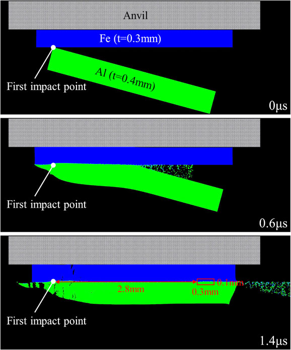
Figure 12 shows the formation process of the wavy interface between 1.05∼1.17 µs in the region inside the dashed line in Fig. 11. While Al obliquely collides with Fe, metal jets are continuously emitted from the collision point. A trigger-like wavy interface is formed behind the collision point. In the emitted metal jets, Al and Fe were randomly mixed and dispersed. In addition, six gauge points (A–F) are selected to investigate the change history of material parameters at the specific location. Gauge points A, C are installed on the surface region (0∼4 µm away from metal surface) of Fe while B, D are installed on the surface region of Al. E and F are installed 20 µm away from the metal surface. During the collision process, A and B were drawn into the apex of the wavy interface. C and D moved to the foot of wave. E and F installed at locations far from the interface did not move much from the initial position compared to other gauge points and remained in each base metal away from the interface throughout the collision process.

To further confirm the component of metal jet, two different colors are assigned to the surface region of each metal plates (as shown in Fig. 13). The yellow and purple particles are indicating the region 5 µm from the surface of parent plate and flyer plate, respectively. The numbers of Al and Fe particles in the emitted metal jets in Fig. 13 were counted and the particle number ratio of Al and Fe was about 26:1. It clearly shows that the emitted metal jets mainly composed of Al. Kakizaki et al.15) compared the composition of the metal jet at different metal density differences using both simulation and experiment methods. They proved that when the density difference of the two metal plates was large (Al/Cu, Al/Fe, Al/Ni), the metal jet mainly composed of the lower density metal. When the density between each metal is close (Al/Al, Cu/Ni), the metal jet composed of both metals with a similar amount. This can be explained by the conservation of momentum during collision process in MPW. An ideal situation describing the impact process at one unit distance ΔX is assumed without considering the friction loss and air resistance (Fig. 14). In this ideal situation, the total momentum is assumed to be conserved for both the whole flyer-parent plate system and local collision at one unit distance ΔX. The flyer plate firstly impacts onto the parent plate with an impact velocity of v, then the two plates are joined and keep moving with a buffered velocity v′ in a short time. The points A and B are the center of gravity of the flyer plate and parent plate before the impact, while A′ and B′ show the center of gravity after the impact. The thickness of each plate is reduced due to compression caused by the plastic deformation. The center of gravity of each plate is moving upward and the distance changes are indicated by df and dp, respectively. According to the conservation of momentum, for unit distance ΔX during the collision process in MPW, there is:
| \begin{equation}
(m_{\text{f}} + m_{\text{p}})v' - m_{\text{f}}v = 0
\end{equation}
| (1) |
| \begin{equation}
(m_{\text{p}})v' = F\varDelta t, \quad m_{\text{f}}(v' - v) = F \varDelta t
\end{equation}
| (2) |
where
mf and
mp are the mass of flyer plate and parent plate per unit area, they are determined by the thickness of each plate and the density of each material;
F is the interaction force applied on each plate. For each SPH particle with same volume, The
eq. (1) can be rewritten as:
| \begin{equation}
\rho_{\text{f}}\Delta v_{\text{f}} + \rho_{\text{p}}\Delta v_{\text{p}} = 0
\end{equation}
| (3) |
The
eq. (3) shows that particles with lower density have a larger change in velocity, therefore lighter particles are more likely to be ejected as metal jet.


The relationship between the emission behavior of the metal jet near the collision point and the formation of the wavy interface will be investigated in more detail. Figure 15 shows the emission behavior of metal jet near the collision point from 1.07∼1.12 µs. At 1.07 µs, the metal jets were emitted from the Al side toward the Fe surface in front of the collision point. The emitted metal jets collide with the Fe surface in front of the collision point at 1.08 µs, and most of them were emitted as an Emitted flow along the Fe surface in front of the collision point, and a part of them were incorporated into the interface as an Entrapped flow. Furthermore, as shown by the yellow arrow, Fe overhangs to the Al side, causing a flow of Fe particles in the opposite direction to the Entrapped flow. As a result, an apex between Al and Fe was formed behind the collision point at 1.09 µs. At 1.10 µs, the overhang of Fe occurred in the region indicated by the yellow arrow, and the emission direction of the metal jet changed toward the Fe surface in front of the collision point. At 1.11 µs, the metal jet collides with the Fe surface again. At this time, as in 1.08 µs, the metal jets divided into the Emitted flow emitted along the Fe surface in front of the collision point and the Entrapped flow incorporated into the interface, and the latter formed an apex between Al and Fe. At 1.12 µs, as in 1.09 µs, an apex between Al and Fe was formed behind the collision point due to the flow of Fe particles in the opposite direction to the Entrapped flow as indicated by the yellow arrow. In this way, in the Al/Fe magnetic pulse welding, the metal jets are emitted from the Al side with low density and repeatedly collide with the Fe surface with high density in front of the collision point, resulting in a trigger-like wavy interface.

Figure 16 shows the pressure change at each gauge point during the formation of a wavy interface. The pressure at gauge points A and B located at the apex of wave within Al and Fe increase rapidly to 25 GPa and 9 GPa around 1.1 µs. After that, the pressure decreases gradually until 1.4 µs. The rapid increase in pressure is expected to cause large compression. The pressure of gauge point C and D, where located at the foot of wave, reached around 18 GPa and 5 GPa, respectively.

The maximum pressure of A, C are higher than B, D, which indicates that the location of A and C in Fe experienced more compression than B and D in Al. During the collision, the pressure at the outermost surface of the colliding metal plate should be the same due to the interaction, but due to the low density of Al, more particles on the outermost surface of the Al plate are emitted as metal jets. Therefore, the Fe particles left at the apex of wavy interface after the collision is almost the same Fe on the outermost surface of the Fe plate, while the Al left at the apex of wavy interface is not the same Al on the outermost surface of the Al plate. Therefore, the maximum pressure of Fe in the apex of wave within Fe is considered higher than that of Al.
In addition, the maximum pressure at E and F where located far away from interface were smaller than that of A–D, and the maximum pressure was about 3∼4 GPa. Therefore, the compression at E and F are smaller than that of A–D. It should be noted that the pressure increased rapidly due to the collision, but then also dropped rapidly. At 1.4 µs, the pressure at all gauge points dropped to almost atmospheric pressure. In this way, it was clarified that the time when the high pressure is reached near the joint interface during collision is extremely short.
As the pressure increases, the melting point of the material is expected to increase as well.16,17) Therefore, to discuss local melting phenomenon at the joint interface, it is necessary to consider not only the temperature increase at the joint interface during collision, but also the increase in the melting point of the material due to the increase in pressure at the collision point. In 1966, Gilvarry simplified Lindemann’s equation of melting by approximating it based on data from previous studies and showed that the pressure dependence of the melting point can be expressed by eq. (4).16)
| \begin{equation}
T_{m} = T_{m0}(V_{0}/V)^{2 \varGamma - 2/3}
\end{equation}
| (4) |
where
Tm = melting point under high pressure,
Tm0 = melting point under atmospheric pressure,
V = volume under high pressure,
V0 = volume under atmospheric pressure,
Γ = Grüneisen coefficient. A linear relationship between volume change (
V0/
V) and pressure has been found in many collision experiments.
18) Al and Fe can be expressed
eq. (5) and
(6).
| \begin{equation}
(V_{0}/V)_{\textit{Al}} = 0.0086p + 1
\end{equation}
| (5) |
| \begin{equation}
(V_{0}/V)_{\textit{Fe}} = 0.0055p + 1
\end{equation}
| (6) |
The change in melting point of each metal as the pressure change can be derived by substituting
eq. (5) and
(6) into
eq. (4).
Figure 17 compares the temperature changes and the changes in melting points of Fe and Al estimated from pressure changes at each gauge point. The calculation method of temperature at each particle in the SPH model can be found in the previous report.
11) The black and red lines in the figure show the temperature and the melting point that changes with increasing pressure.
The temperature at each gauge point reached its maximum around 1.1 µs. The maximum temperatures of A and B increased rapidly to about 2600 K and 1730 K at around 1.1 µs, respectively. The maximum temperature of C and D reached 1930 K and 1130 K. The temperatures of E and F located away from the joint interface hardly changed. According to Gauss’s law, the magnetic flux generated in the coil is attenuated by the square of the distance, so it is considered that the direct effect of the leakage magnetic field of the coil on the temperature rise at the interface is extremely small.
The melting point increased up to about 2610 K and 1060 K for A and B, respectively, as the pressure increased near 1.1 µs. The melting points at C and D increased to about 2340 K and 1030 K, respectively. And the melting points at E and F increased to about 1910 K and 980 K, respectively. Among these selected gauge points, the temperature at A and B has clearly exceeded the melting point of Fe and Al, respectively. Therefore, it is considered that melting occurs at the location of A and B. Although the highest temperature at C (1930 K) passed the atmospheric melting point of Fe (1811 K), it did not exceed the melting point at the corresponding high pressure (2340 K). So, the local melting did not occur at C. The temperature at C exceeded the melting point by a little amount, but not as much as B. Therefore, local melting is also considered occur at location D to a lesser degree than B. The temperatures at E and F have not reached the melting point, and it is considered that melting does not occur at these locations.
In this way, the melting points of Fe and Al increase due to the increase in pressure caused by the collision. However, these increased melting points decreased rapidly when the pressure returns to atmospheric pressure, and at 1.4 µs, they became almost equal to the melting point under atmospheric pressure.
4.5 Temperature distribution and location of local melting zone at the joint interface
Figure 18(a) shows the temperature distribution of the wavy interface at 1.4 µs. The temperature of the base metal of Fe remained at room temperature of 300 K and hardly increased at more than 30 µm from the interface. On the Al side, the temperature rose to about 400∼700 K within 40 µm from the interface, but the temperature of the base metal further away from the interface did not rise and remained at 300 K, as in the case of Fe. In addition, high temperature regions exceeding 1500 K have been observed near the apex region, where the melting of Fe and Al may occur. Therefore, such region is defined as local melting zone (LMZ). Figure 18(b) shows the location of LMZ (as indicated in red color). Local melting phenomenon is limited to the extreme vicinity of the joint interface. Therefore, it is considered that a large temperature difference occurs between the joint interface and the base metal where temperature has hardly risen, and this large temperature difference causes rapid heat removal.

To clarify the formation mechanism of IML formed at the joint interface and its formation process, it is necessary to investigate the cooling process of the joint interface in detail in addition to the temperature and substance distribution at the joint interface clarified in this study. However, the simulation method used in this study cannot reproduce the cooling process of the joint interface. To achieve this purpose, it is necessary to introduce an analysis method that can analyze heat conduction. Therefore, we also investigated the cooling process of the joint interface using OpenFOAM. The results of the study on the formation process of IML based on the cooling process of the joint interface will be reported in a separate report.
It is worth noting that the SPH method can calculate the local composition from the ratio of particles in a certain region, and from the obtained temperature change and material, it can calculate the composition of the IML, which is considered to be formed by partial melting and rapid cooling, such as TSL. However, it cannot reproduce the fragments ejected from Fe surface by the impact as far as the SPH model assuming a smooth sample surface is analyzed. It is possible to reproduce even finer parts of the wavy interface by reducing the size of h. In addition, more precise observation is required to trace the movement of particles and their time-dependent changes in location, temperature in the jet and the heavily deformed area surrounding the collision point.


