Relationship between the calcaneal size and body mass in primates and land mammals

Abstract

The relationship between calcaneal size and body mass in extant primates and other land mammals is examined using regression analyses to provide simple equations for estimating the body mass of extinct primate and land mammal species based on the calcaneus. The results imply that among the linear calcaneal dimensions, the calcaneal width at the talar articular surfaces (CA2) is likely the best body mass estimator for land mammals (including primates), and the width of the posterior talar articular surface (CA3) appears to be relatively good body mass estimator for primates. The equation with a 95% prediction interval for estimating the body mass (BM, in g) using CA2 (in mm) for land mammals is: BM = exp(2.928 × ln CA2 + 0.981 ± 0.772) × 1.076; the corresponding equation using CA3 (in mm) for primates is: BM = exp(2.555 × ln CA3 + 3.536 ± 0.641) × 1.067.

Introduction

The heelbone (calcaneus or calcaneum) and anklebone (talus or astragalus) of primates and other mammals have been well studied in primatology, anthropology, archaeozoology, and vertebrate paleontology as indicators of functional adaptation, phylogeny, and taxonomy (e.g. Szalay, 1977; Gebo et al., 1991; Dagosto and Terranova, 1992; Ciochon et al., 2001; Ciochon and Gunnell, 2004; Gebo and Dagosto, 2004; Gunnell and Ciochon, 2008; Polly, 2008; Marivaux et al., 2010; Jogahara and Natori, 2013; Tsubamoto, 2014; Tsubamoto et al., 2016 and references therein). The bony structure and shape of these two bones are relatively compact and robust (e.g. Gray, 1858), so that these bones are frequently preserved and are found undamaged more often than long bones, vertebrae, or fragile skulls in the fossil and zooarchaeological assemblages (Tsubamoto, 2014; Tsubamoto et al., 2016). The body mass of primates and other mammals, on the other hand, is a useful predictor of species adaptations and diversities because it is strongly correlated with many aspects of life history, ecology, and behavior, etc. (e.g. Peters, 1983; Calder, 1984; LaBarbera, 1989). Therefore, estimates of the body mass of extinct mammalian species play an important role in paleoecological, paleoprimatological, and physical anthropological analyses (e.g. Legendre, 1986, 1989; Conroy, 1987; Anyonge, 1993; Fleagle, 1999; Egi, 2001; Smith et al., 2010; Grabowski et al., 2015; Jungers et al., 2016; Tsubamoto et al., 2016; Ruff and Niskanen, 2018 and references therein). Several studies have investigated the relationship between talar size and body mass in primates and other mammals (Dagosto and Terranova, 1992; Martinez and Sudre, 1995; Rafferty et al., 1995; Polly, 2008; Parr et al., 2011; Tsubamoto, 2014; Yapuncich et al., 2015; Tsubamoto et al., 2016; Dagosto et al., 2018). However, only a few studies have investigated the relationship between calcaneal size and body mass: for example, Dagosto and Terranova (1992) did it for ‘prosimian’ primates (strepsirrhines and Tarsius); Yapuncich et al. (2015) did it for euarchontans (primates, scandentians, and dermopterans); and Dagosto et al. (2018) did it for euarchontans and small mammals.

In this material report, the relationships between the calcaneal size and body mass in living primates and land mammals are examined using regression analyses. The purpose of this report is to provide simple equations that will allow paleoprimatologists and vertebrate paleontologists to estimate the body masses of extinct primate and land mammal species from the calcaneal size. The original data used here are limited, and hence this report should be treated as a pilot study simply for the body mass estimation from the calcaneus. Any other functional signals for, for example, behavior and ecology are not discussed here.

Materials and Methods

The original data used in this study consist of the body mass and 12 linear measurements of the calcaneus of superficially 69 individuals, representing 44 species belonging to 10 orders of extant land mammals, and ranging in body mass from 18 g to 1.4 tonnes (Table 1). Most of the samples are adult individuals with three subadult specimens. These three subadult specimens (Table 1) are used to increase the data points. Most of the individuals used here are the same individuals used by Tsubamoto (2014) and Tsubamoto et al. (2016). The body masses represent the actual body weight of the individual of each specimen and were recorded either while the animals were still alive or just after their death (Tsubamoto, 2014). The data (body mass and 12 linear measurements) for the adult males and females of Japanese monkey (Macaca fuscata fuscata: Primates, Cercopithecidae) and Japanese raccoon dog (Nyctereutes procyonoides viverrinus: Carnivora, Canidae) were derived from the mean values of more than 25 specimens for each sex of each species (Table 1). Owing to the limited availability of specimens for which such data could be obtained, the dataset is somewhat biased towards primates and carnivores (Table 1; Tsubamoto, 2014). The 12 linear measurements (CA1–CA12) are indicated in Figure 1 and Table 2. The units of the linear measurements and body mass are in millimeters (mm) and grams (g), respectively (Table 1).

Table 1 The original data used in this paper

Higher taxa	Specimen no.	Species	BM (g)	Sex	CA1	CA2	CA3	CA4	CA5	CA6	CA7	CA8	CA9	CA10	CA11	CA12
Primates	NSM-M 31595	Gorilla gorilla	216000	M	95.89	50.57	28.25	25.05	39.99	45.92	33.36	31.76	23.89	41.66	36.10	49.42
Primates	KUPRI 8135	Hylobates agilis	8000	F	27.71	15.31	8.26	7.12	8.15	8.44	11.17	9.91	7.53	13.94	13.94	17.63
Primates	NSM-M 32559	Pan troglodytes	50000	F	53.83	32.41	18.46	18.22	19.37	20.13	25.58	22.99	14.16	30.60	25.69	30.46
Primates	NSM-M 33042	Pan troglodytes	43600	F	54.39	32.72	18.17	17.78	19.74	21.48	22.47	22.71	15.42	29.94	24.81	29.86
Primates	NSM-M 31996	Pongo pygmaeus	61000	F	58.35	31.81	16.36	11.48	14.88	20.76	20.74	19.52	14.87	25.14	22.17	30.61
Primates	KUPRI 4237	Erythrocebus patas	5000	F	33.38	14.31	7.40	6.44	9.59	12.18	8.87	10.05	7.43	13.27	10.10	11.52
Primates	*	Macaca fuscata	10245	M	38.05	17.35	9.28	8.78	11.66	13.63	11.75	12.52	8.87	16.25	14.05	16.89
Primates	**	Macaca fuscata	7119	F	34.46	15.96	8.45	7.66	10.47	12.03	10.86	11.39	8.15	14.73	12.88	15.36
Primates	KUPRI 1626	Papio anubis	31400	M	48.44	23.97	13.91	13.99	17.10	17.93	16.30	17.22	13.19	23.34	21.10	22.55
Primates	KUPRI 1625	Papio anubis	29400	M	51.94	26.93	14.47	13.51	17.74	18.36	17.57	16.92	13.29	24.88	22.20	24.19
Primates	KUPRI 307	Papio anubis	42000	M	50.28	25.68	14.29	13.70	16.94	19.48	14.56	16.76	12.10	23.67	20.42	23.74
Primates	KUPRI 2779	Papio hamadryas	10200	F	37.31	18.75	9.68	8.41	12.63	12.54	13.09	12.82	9.53	16.78	13.97	16.66
Primates	KUPRI 6077 (subadult)	Papio hamadryas	18100	M	48.48	22.93	12.67	11.77	16.83	16.70	12.77	15.95	11.83	20.19	16.96	18.39
Primates	KUPRI 6449	Aotus trivirgatus	940	M	20.52	8.64	4.13	3.95	5.20	6.31	6.69	5.82	4.85	8.39	7.53	8.49
Primates	KUPRI 7125	Aotus trivirgatus	1064	F	19.39	8.29	4.20	3.84	5.12	5.16	6.12	5.65	4.36	8.35	7.51	8.48
Primates	KUPRI 7130	Callithrix jacchus	300	F	11.45	5.49	2.56	2.94	3.27	3.16	3.71	3.74	2.56	4.90	4.12	4.46
Primates	KUPRI 6424	Callithrix jacchus	382	M	11.23	4.46	2.29	2.35	3.06	3.48	3.36	3.12	2.53	4.73	4.01	4.09
Primates	KUPRI 4487	Callithrix jacchus	460	M	10.66	4.17	2.44	2.27	2.56	2.49	3.76	3.14	2.32	4.43	3.75	4.22
Primates	KUPRI 6091	Cebus apella	2600	F	24.55	10.37	5.18	4.54	6.90	7.32	7.31	7.09	5.64	8.80	7.85	8.55
Primates	KUPRI 4245	Cebus apella	2200	M	26.64	12.77	5.98	6.19	7.82	8.24	8.94	8.89	5.92	10.56	8.81	10.41
Primates	KUPRI 6429	Saguinus midas	400	M	13.78	5.67	3.15	2.56	3.18	3.32	4.52	3.94	2.82	5.45	4.35	4.71
Primates	KUPRI 4314	Saguinus midas	550	F	13.60	5.96	3.05	2.39	3.41	3.95	4.46	4.09	2.71	5.22	4.12	4.68
Primates	KUPRI 7174	Saguinus oedipus	450	M	14.56	6.04	2.60	2.63	3.34	4.16	4.39	4.32	2.88	5.42	4.42	4.74
Primates	KUPRI 4282	Saimiri sciureus	700	M	16.53	7.10	3.16	3.40	4.56	4.27	5.09	5.09	3.66	6.66	5.66	5.79
Primates	KUPRI 3908	Saimiri sciureus	540	F	17.14	7.07	3.20	3.20	3.99	4.84	5.78	5.22	3.92	6.83	5.92	6.64
Primates	KUPRI 4691	Galago crassicaudatus	910	M	33.26	6.89	2.78	3.21	4.77	8.13	4.61	5.27	4.05	7.26	5.75	6.54
Primates	KUPRI 4315	Galago senegalensis	100	F	25.99	4.30	1.77	2.05	2.87	4.44	2.90	2.44	2.15	4.37	3.78	4.18
Primates	KUPRI 6699	Lemur catta	2330	F	24.09	10.22	3.86	5.25	6.56	6.97	6.41	7.40	5.02	9.79	8.79	9.28
Scandentia	KUPRI 2789	Tupaia glis	125	F	9.20	4.71	1.73	1.78	2.39	3.18	2.69	2.62	1.94	3.52	2.71	2.99
Scandentia	KUPRI 2914	Tupaia glis	90	F	8.73	4.20	1.49	1.57	2.20	2.96	2.53	2.61	1.91	3.27	2.56	2.90
Carnivora	NSM-M 31458	Ailuropoda melanoleuca	108300	F	61.64	28.87	10.97	12.27	22.64	28.55	24.81	17.87	13.75	26.62	19.85	25.24
Carnivora	KUPRI-Z 441	Canis familiaris	5690	F	33.29	13.20	6.24	5.73	9.89	14.34	11.03	10.52	7.69	14.16	9.42	10.71
Carnivora	KUPRI-Z 438	Canis familiaris	14500	M	39.30	15.23	7.26	6.91	11.25	15.75	12.94	11.40	8.70	17.22	11.14	11.82
Carnivora	KUPRI-Z 986	Felis catus	3300	?	28.72	11.08	4.81	5.10	7.35	10.75	9.21	5.01	6.94	10.07	7.58	7.74
Carnivora	KUPRI-Z 753	Felis catus	6160	M	30.50	11.82	4.69	5.79	7.89	13.08	9.34	5.29	7.14	10.82	8.80	8.03
Carnivora	KUPRI-Z 462	Martes melampus	900	?	18.55	9.29	3.94	3.02	5.23	6.07	8.10	4.38	4.93	7.09	5.76	6.18
Carnivora	KUPRI-Z 460	Martes melampus	900	F	16.97	8.65	3.68	2.85	4.91	6.54	6.97	4.25	5.01	6.47	5.43	5.62
Carnivora	KUPRI-Z 619	Mustela sibirica	300	M	9.90	4.52	1.99	1.64	2.74	3.31	3.66	2.68	2.60	3.98	3.39	4.03
Carnivora	KUPRI-Z 620	Mustela sibirica	150	F	7.20	3.44	1.46	1.26	2.23	3.79	1.83	1.77	1.99	2.81	2.57	3.10
Carnivora	KUPRI-Z 621	Mustela sibirica	420	M	12.48	6.19	3.18	2.59	4.24	3.96	5.14	3.58	2.88	5.47	5.02	5.83
Carnivora	***	Nyctereutes procyonoides	3651	M	23.94	10.38	4.28	4.23	6.45	9.93	8.31	6.96	5.70	9.90	7.36	9.04
Carnivora	****	Nyctereutes procyonoides	3805	F	23.77	10.39	4.20	4.21	6.35	9.80	8.38	7.02	5.81	9.80	7.35	8.77
Carnivora	KUPRI-Z 985	Paguma larvata	3600	F	23.24	9.71	4.41	3.17	7.31	8.42	8.07	6.79	5.23	8.02	7.44	7.69
Carnivora	KUPRI-Z 1376 (subadult)	Paguma larvata	3400	F	24.92	10.08	4.05	3.44	6.42	9.08	8.67	7.14	5.60	8.29	7.82	8.33
Carnivora	NMS-M 31999 (subadult)	Pantela leo	131000	M	107.26	39.85	16.60	18.50	30.07	53.73	32.15	25.25	20.75	43.20	31.98	31.60
Carnivora	NSM-M 33055	Pantela leo	97000	F	90.16	36.24	13.69	15.58	24.81	42.18	27.80	21.47	18.15	38.30	31.59	24.94
Carnivora	KUPRI-Z 747	Procyon lotor	6100	F	28.93	12.94	4.89	5.07	8.26	9.21	10.43	7.70	7.64	11.08	8.98	10.39
Carnivora	KUPRI-Z 767	Suricata suricatta	450	?	15.05	6.01	2.64	2.53	4.43	4.97	4.67	3.13	3.88	5.59	4.78	5.21
Carnivora	NSM-M 33061	Ursus actos yesoensis	163200	F	81.94	45.51	18.80	17.15	29.69	41.67	32.69	26.42	20.14	42.25	33.45	35.37
Carnivora	KUPRI-Z 403	Vulpes vulpes	4700	M	31.90	12.77	5.11	5.31	8.09	14.00	10.16	9.29	7.83	12.78	9.27	9.86
Carnivora	KUPRI-Z 414	Vulpes vulpes	3900	F	30.33	11.53	4.90	5.10	7.92	12.14	10.33	5.65	7.17	11.96	8.73	8.91
Eulipotyphla	NSM-M 20690	Urotrichus talpoides	18	F	3.76	1.54	0.67	0.57	0.64	1.99	0.77	0.74	0.64	1.10	1.03	1.10
Rodentia	NSM-M 35524	Cavia porcellus	550	F	13.09	5.86	2.54	2.54	2.75	3.17	3.60	2.88	2.30	4.25	2.68	3.54
Lagomorpha	KUPRI-Z 785	Lepus brachyurus	3000	M	27.14	11.26	4.25	5.58	7.13	11.65	6.61	7.93	5.19	9.40	5.14	4.81
Lagomorpha	KUPRI-Z 787	Lepus brachyurus	2150	F	27.42	11.54	4.41	5.12	6.62	12.30	7.17	7.92	3.67	10.07	5.39	5.58
Tubulidentata	NSM-M 34334	Orycteropus afer	49300	M	75.68	35.62	14.81	14.28	17.15	42.19	19.36	32.68	19.40	34.93	25.97	26.89
Artiodactyla	KUPRI-Z 1331	Cervus nippon	35000	F	66.33	22.43	6.34	6.92	14.28	43.11	14.88	16.77	8.59	23.49	16.04	18.60
Artiodactyla	NSM-M 33056	Bubalus babalis	513000	M	156.59	54.88	21.18	25.78	42.72	101.09	32.02	15.40	43.02	67.44	39.14	49.37
Artiodactyla	NSM-M 31301	Bubalus babalis	374400	F	143.39	50.07	19.05	22.27	39.17	89.82	30.50	16.31	42.88	57.71	34.69	43.03
Artiodactyla	NSM-M 31304	Giraffa camelopardalis	800000	M	192.06	77.57	25.99	31.18	51.72	123.99	43.58	21.02	54.05	91.03	51.03	53.35
Artiodactyla	NSM-M 33057	Giraffa camelopardalis	620000	F	184.80	73.78	22.86	32.17	53.33	114.17	45.16	23.41	56.42	87.53	49.61	59.00
Artiodactyla	NSM-M 31318	Oryx dammah	99000	M	94.47	33.22	9.34	12.62	25.10	63.23	20.78	13.16	24.91	37.08	25.17	26.67
Perissodactyla	NSM-M 33530	Ceratotherium simum	1400000	F	129.50	81.45	44.32	45.66	56.34	73.11	38.60	35.68	37.24	66.00	57.22	78.25
Perissodactyla	NSM-M 31302	Equus ferus przewalskii	357400	F	101.59	53.38	23.64	18.33	30.72	57.16	22.75	13.23	21.54	46.36	40.65	49.98
Perissodactyla	NSM-M 31303	Equus ferus przewalskii	345100	F	105.95	52.46	22.72	19.75	32.84	57.37	23.75	13.72	19.04	47.35	39.36	50.33
Perissodactyla	NSM-M 33398	Equus grevyi	295400	F	107.14	53.66	22.66	19.06	30.83	56.87	18.68	12.24	19.02	47.51	43.01	50.98
Perissodactyla	NSM-M 31634	Tapirus indicus	297900	M	111.49	51.99	22.95	15.99	29.07	59.96	24.36	17.59	30.53	41.50	32.91	40.44
Perissodactyla	NSM-M 33067	Tapirus terrestris	237700	F	101.08	45.66	26.13	18.19	24.97	52.62	23.93	14.69	27.34	36.21	30.88	35.92
Marsupialia	NSM-M 35838	Macropus giganteus	56200	M	80.03	25.64	11.72	17.44	23.08	57.15	14.91	25.07	22.93	28.96	23.92	26.31

Institutional abbreviations: KUPRI, Primate Research Institute, Kyoto University, Inuyama, Japan; KUPRI-Z, zoological collection stored in KUPRI; NSM-M, mammalian collection stored in National Museum of Nature and Science, Tsukuba, Japan (formerly National Science Museum, Tokyo, Japan). Other abbreviations: BM, body mass; M, male; F, female; CA1–CA12, linear measurements of the calcaneus used in this study (in mm; Figure 1; Table 2).

*  Data from the mean values of 110 adult male specimens of Macaca fuscata stored in KUPRI.

**  Data from the mean values of 119 adult female specimens of M. fuscata stored in KUPRI.

***  Data from the mean values of 35 adult male specimens of Nyctereutes procyonoides stored in KUPRI.

****  Data from the mean values of 28 adult female specimens N. procyonoides stored in KUPRI.

Figure 1

Twelve linear measurements (CA1–CA12) made on the calcaneus used in this study. The definitions of CA1–CA12 are shown in Table 2. The illustrations are based on a left calcaneus of Macaca fuscata (Primates, Catarrhini, Cercopithecidae): (A) dorsal (anterior) view; (B) lateral view; (C) distal view.

Table 2 Definitions of the 12 linear measurements (CA1–CA12; Figure 1) of the calcaneus

Measurement	Definition
CA1	calcaneal length (= C1 of Dagosto and Terranova, 1992)
CA2	calcaneal width at the talar articular surfaces (~C2 of Dagosto and Terranova, 1992)
CA3	width of the posterior talar articular surface (= C4 of Dagosto and Terranova, 1992)
CA4	width of the posterior calcaneal body
CA5	width of the tuberosity
CA6	length of the posterior calcaneal body (= C7 of Dagosto and Terranova, 1992)
CA7	length of the posterior talar articular surface (= C3 of Dagosto and Terranova, 1992)
CA8	width of the articular surface for cuboid (= C6 of Dagosto and Terranova, 1992)
CA9	height of the articular surface for cuboid (= C5 of Dagosto and Terranova, 1992)
CA10	height at the posterior talar articular surface
CA11	height at the posterior calcaneal body
CA12	height at the tuberosity

The data were transformed to natural logarithms for the analyses. The regression analyses were performed using the same procedure used by Tsubamoto (2014) and Tsubamoto et al. (2016). They were performed on two data sets: the land mammal model (superficially 69 individuals; including primates) and primate model (superficially 28 individuals) (Table 1, Table 3).

Table 3 Summary of bivariate simple regression analyses performed using Excel (Microsoft) to predict the body mass on a natural log scale

		ln CA1	ln CA2	ln CA3	ln CA4	ln CA5	ln CA6	ln CA7	ln CA8	ln CA9	ln CA10	ln CA11	ln CA12
Land mammal model	Slope	2.969	2.928	2.857	2.815	2.747	2.359	3.074	3.027	2.757	2.779	2.861	2.777
N = 69	Intercept	−1.611	0.981	3.486	3.629	2.718	2.773	1.788	2.390	3.227	1.600	2.041	1.917
t-value = 1.9960	SEE	0.649	0.387	0.639	0.609	0.441	0.674	0.660	1.064	0.571	0.441	0.522	0.551
(df = 69 – 2 = 67)	adjusted R2	0.941	0.979	0.943	0.948	0.973	0.936	0.939	0.841	0.954	0.973	0.962	0.957
(95% CL)	adjusted CF	1.156	1.076	1.203	1.161	1.116	1.092	1.342	1.876	1.037	1.061	1.205	1.165
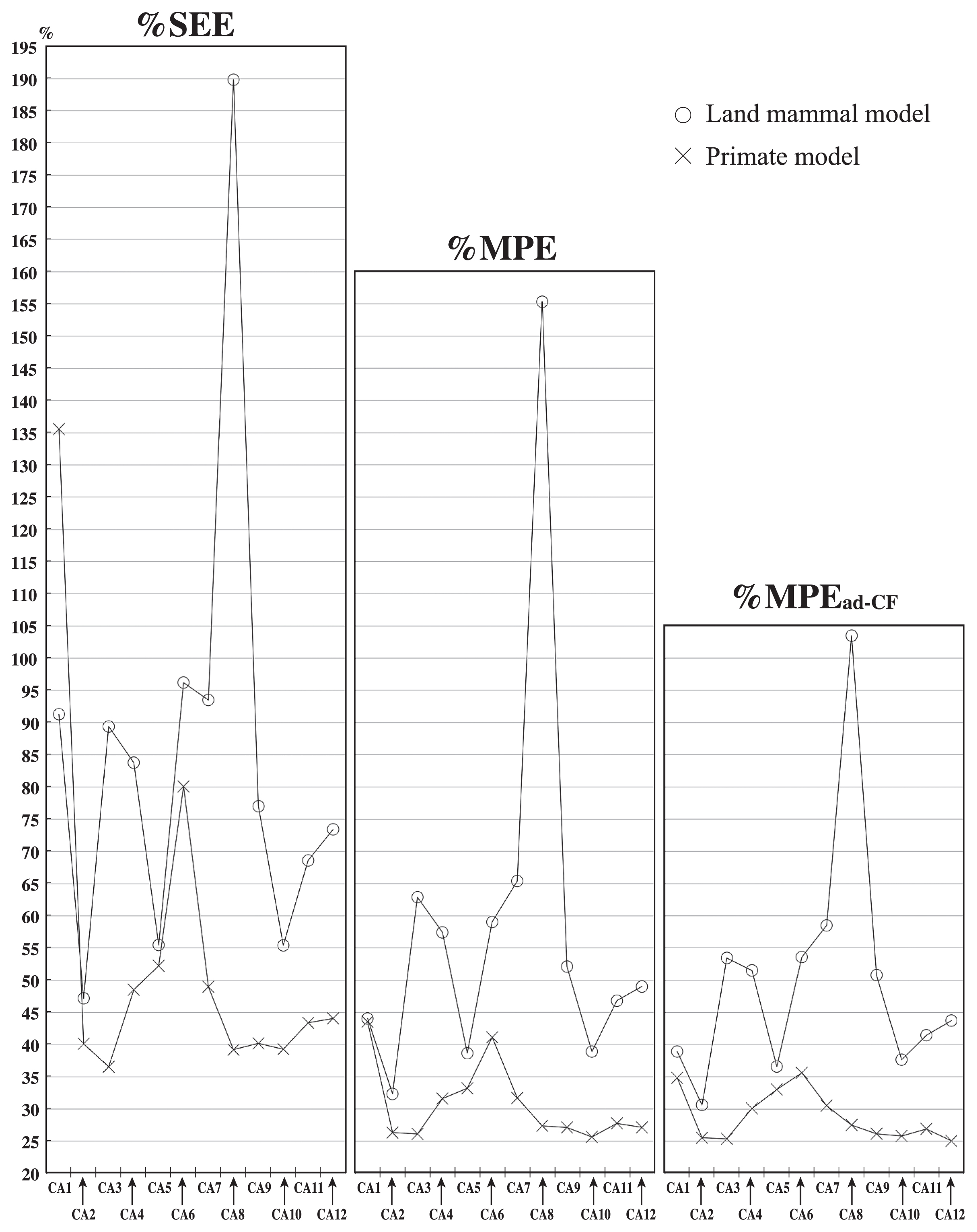
	%SEE	91.293	47.210	89.396	83.779	55.458	96.225	93.515	189.815	77.019	55.415	68.611	73.418
	%MPE	44.075	32.360	62.890	57.423	38.673	59.048	65.407	155.350	52.109	38.924	46.841	49.036
	%MPEad-CF	38.925	30.649	53.452	51.509	36.592	53.591	58.515	103.496	50.793	37.654	41.462	43.755
Primate model	Slope	3.153	2.782	2.555	2.678	2.656	2.617	2.957	2.836	2.891	2.938	2.871	2.690
N = 28	Intercept	−2.325	1.213	3.536	3.424	2.756	2.527	1.834	2.139	2.914	1.038	1.649	1.704
t-value = 2.0555	SEE	0.857	0.337	0.312	0.396	0.420	0.588	0.399	0.331	0.338	0.331	0.361	0.365
(df = 28 – 2 = 26)	adjusted R2	0.823	0.973	0.977	0.962	0.957	0.917	0.962	0.974	0.972	0.974	0.969	0.968
(95% CL)	adjusted CF	1.331	1.071	1.067	1.074	1.029	1.098	1.045	1.103	1.092	1.077	1.101	1.064
	%SEE	135.574	40.135	36.565	48.535	52.244	80.102	48.991	39.223	40.210	39.299	43.408	44.079
	%MPE	43.558	26.349	26.139	31.626	33.218	41.161	31.717	27.412	27.144	25.677	27.780	27.157
	%MPEad-CF	34.847	25.552	25.390	30.094	33.046	35.604	30.527	27.520	26.167	25.828	26.928	25.059

Abbreviations: N, sample size; SEE, standard error of estimate; adjusted R², coefficient of determination adjusted to the number of variables; adjusted CF, correction factor adjusted using the three correction factors proposed by Tsubamoto (2014); df, degrees of freedom; CL, confidence level; %SEE, percent standard error of estimate; %MPE, mean percentage prediction error; %MPE_ad-CF, %MPE for the corrected values using the adjusted CF (Tsubamoto, 2014). Bold value with underline indicates the lowest value in each row of %SEE, %MPE, and %MPE_ad-CF; bold value indicates the second lowest value in it; and value with underline indicates the third lowest value in it.

The results of the multiple regression analysis with a stepwise option performed using the JMP package (SAS Institute Inc.) vary according to the criteria used in the software. Therefore, here, simple linear bivariate regression analysis was applied to perform the body mass estimation. Although multiple regression analysis or areal/volumetric regression analysis may provide more ‘accurate’ equations, I chose simple linear regression analysis to provide simpler equations and to extend the availability and applicability of the equations for vertebrate paleontologists. On the other hand, although Model II regression techniques such as major axis and reduced major axis regressions are sometimes used for body mass estimation (e.g. Egi, 2001; Niskanen et al., 2018; Ruff and Niskanen, 2018; Ruff et al., 2018), I chose the least-squares regression because it can provide prediction errors (Warton et al., 2006).

When regression is performed using log-transformed data, a systematic detransformation bias is introduced (Smith, 1993a, b). To correct for this bias, correction factors are sometimes used (Sprugel, 1983; Snowdon, 1991; Smith, 1993a, b; Egi et al., 2002, 2004; Tsubamoto, 2014; Tsubamoto et al., 2016). Here, the adjusted correction factor (adjusted CF) proposed by Tsubamoto (2014) was calculated (Table 3) and applied. When estimating body mass, the estimated log value of the body mass is first de-transformed to the actual value in grams, and then is multiplied by the adjusted CF (Tsubamoto, 2014).

For the body mass estimation process, the 95% prediction intervals were calculated. The approximations of the 95% prediction intervals can be calculated as follows using the standard error of estimate (SEE) (Ruff, 2003; Tsubamoto, 2014; Tsubamoto et al., 2016): ± t-value × SEE. This approximation was used here to calculate the estimated body masses easily. The estimated body mass (BM in the equation) with 95% prediction interval for the measurements using the adjusted CF is calculated as follows: BM in g = {exp[slope × ln(measurement in mm) + intercept (± t -value × SEE )> × adjusted CF.

The degree of correlation (accuracy) between body mass and calcaneal size was evaluated using the percent standard error of estimate (%SEE) and the mean percentage prediction errors (%MPE and %MPE_ad-CF) (Tsubamoto, 2014; Tsubamoto et al., 2016). %SEE for natural log-transformed data was calculated as %SEE = (e^SEE – 1) × 100 (Smith, 1984a; Egi et al., 2002; Ruff, 2003). %PE is the percentage of prediction error of the de-transformed value (not using the adjusted CF) and is calculated as %PE = (original value – estimated value)/estimated value × 100 (Smith, 1981, 1984a, b). %MPE is the arithmetic mean of the absolute values of %PE for each variable calculated for each individual (Smith, 1981, 1984a, b; Dagosto and Terranova, 1992). %MPE_ad-CF is %MPE for the values corrected using the adjusted CF (Tsubamoto, 2014).

Results and Remarks

The results of the simple bivariate regression analyses are shown in Table 3 and in Figure 2 and Figure 3. The values of the degree of correlation for the measurements (%SEE, %MPE, and %MPE_ad-CF) vary in each model.

Figure 2

Comparison of %SEE, %MPE, and %MPE_ad-CF of the body mass estimate regressions derived from the calcaneal dimensions (Figure 1; Table 2).

Figure 3

Examples of body mass (BM; in g) estimate regressions and data scatters on a natural log scale: (A) using CA2 (in mm) for the mammal model; and (B) using CA3 (in mm) for the primate model. Black lines indicate least-squares axis. Dashed lines indicate the upper and lower 95% prediction limits.

In the land mammal model, CA2 has the lowest %SEE, %MPE, and %MPE_ad-CF values (Table 3; Figure 2), i.e. CA2 is the most suitable for the body mass estimation with land mammals as a target, among the 12 measurements. These %SEE, %MPE, and %MPE_ad-CF values (47.21, 32.36, and 30.65, respectively) of CA2 in the land mammal model are higher than those of the best measurement for the body mass estimation based on the talus of land mammals studied by Tsubamoto (2014) (41.98, 28.83, and 28.00, respectively). This implies that the talus is likely better than the calcaneus for body mass estimation with land mammals as a target.

In the primate model, CA3 has the lowest %SEE value and the second lowest %MPE and %MPE_ad-CF values (Table 3; Figure 2). Based on the %MPE and %MPE_ad-CF values of the primate model, CA2 and CA8–CA12 are as low as CA3 (Table 3; Figure 2). Therefore, CA3 appears to be the most suitable for the body mass estimation with the primates as a target, although CA2 and CA8–CA12 are roughly as suitable as CA3. Compared to the values of the good measurements for the body mass estimation in the talus of the primates studied by Tsubamoto et al. (2016), the %SEE value of CA3 of the primate model is lower than that studied by Tsubamoto et al. (2016); and its %MPE and %MPE_ad-CF values are nearly as low as that studied by Tsubamoto et al. (2016). This suggests that, unlike the land mammal model, the calcaneus appears to be as good as the talus for body mass estimation with the primates as a target. However, we should note the fact that the original data of these studies are in fact limited, so that the additional data may alter the results.

The examples of the regression equation with a 95% prediction interval to estimate the body mass (BM, g) are as follows. Using CA2 (in mm) for the land mammal model, BM = exp(2.928 × ln CA2 + 0.981 ± 0.772) × 1.076. Using CA3 (in mm) for the primate model, BM = exp(2.555 × ln CA3 + 3.536 ± 0.641) × 1.067.

The results of the regression analyses of the primate model for CA1–CA3 and CA6–CA9 are briefly compared with those of the calcaneus of the all-strepsirrhine model for the linear measurements C1–C7 by Dagosto and Terranova (1992) (Table 4). The results of CA2–CA3 and CA6–CA9 are roughly similar to those by Dagosto and Terranova (1992). However, the results of CA1 (calcaneal length) are distinguished from those by Dagosto and Terranova (1992): in particular, the slope and intercept are quite different with each other (Table 4). This difference can be information in considering the ecological or phyletic characteristics of the calcaneus of the strepsirrhines among the primates.

Table 4 Comparison of the regressions of the primate model for the linear measurements CA1–CA3 and CA6–CA9 (Figure 1; Table 2) with those of the all-strepsirrhine model for the linear measurements C1–C7 by Dagosto and Terranova (1992)

	This study primate model	Dagosto and Terranova (1992)	This study primate model	Dagosto and Terranova (1992)	This study primate model	Dagosto and Terranova (1992)	This study primate model	Dagosto and Terranova (1992)
	ln CA1	ln C1	ln CA2	ln C2	ln CA3	ln C4	ln CA6	ln C7
Slope	3.15	1.48	2.78	2.86	2.55	3.34	2.62	2.48
Intercept	–2.33	2.13	1.21	1.42	3.54	3.23	2.53	2.70
SEE	0.86	1.16	0.34	0.34	0.31	0.38	0.59	0.70
r	0.95	0.48	0.95	0.97	0.95	0.96	0.95	0.85
%SEE	135.57	218.99	40.14	40.49	36.56	46.23	80.10	101.38
%MPE	43.56	59.32	26.35	26.13	26.14	29.57	41.16	46.36

	ln CA7	ln C3	ln CA8	ln C6	ln CA9	ln C5
Slope	2.96	2.74	2.84	2.70	2.89	2.93
Intercept	1.83	2.35	2.14	2.46	2.91	2.81
SEE	0.40	0.36	0.33	0.28	0.34	0.44
r	0.95	0.96	0.95	0.98	0.95	0.94
%SEE	48.99	43.33	39.22	32.31	40.21	55.27
%MPE	31.72	28.44	27.41	21.05	27.14	32.84

Abbreviations: SEE, standard error of estimate; r, Pearson’s product moment correlation coefficient; %SEE, percent standard error of estimate; %MPE, mean percentage prediction error. CA1: C1 of Dagosto and Terranova (1992); CA2: approximately equal to C2 of Dagosto and Terranova (1992); CA3: C4 of Dagosto and Terranova (1992); CA6: C7 of Dagosto and Terranova (1992); CA7: C3 of Dagosto and Terranova (1992); CA8: C6 of Dagosto and Terranova (1992); CA9: C5 of Dagosto and Terranova (1992).

Acknowledgments

I am grateful to the following individuals involved in access to the specimens used in this research: Masanaru Takai, Takeshi Nishimura, and Naoko Egi (Primate Research Institute, Kyoto University, Inuyama, Japan); and Shin-ichiro Kawada (National Museum of Nature and Science, Tsukuba, Japan). I am also grateful to the reviewer for the useful comments. This work was supported by the Cooperation Program (2011-A-3, 2012-B-2, 2013-B-15, and 2014-B-2) of the Primate Research Institute (Kyoto University, Inuyama, Japan) and by JSPS KAKENHI grant numbers 21770265, 25840172, and 16K07534.

References

•  Anyonge  W. (1993) Body mass in large extant and extinct carnivores. Journal of Zoology, 231: 339–350.
•  Calder  W.A. (1984) Size, Function, and Life History. Harvard University Press, Cambridge.
•  Ciochon  R.L. and  Gunnell  G.F. (2004) Eocene large-bodied primates of Myanmar and Thailand: morphological considerations and phylogenetic affinities. In:  Ross  C.F. and  Kay  R.F. (eds.), Anthropoid Origins: New Visions. Kluwer Academic/Plenum Publishers, New York, pp. 249–282.
•  Ciochon  R.L.,  Gingerich  P.D.,  Gunnell  G.F., and  Simons  E.L. (2001) Primate postcrania from the late middle Eocene of Myanmar. Proceedings of the National Academy of Sciences of the United States of America, 98: 7672–7677.
•  Conroy  G.C. (1987) Problems of body-weight estimation in fossil primates. International Journal of Primatology, 8: 115–137.
•  Dagosto  M. and  Terranova  C.J. (1992) Estimating body size of Eocene primates: a comparison of results from dental and postcranial variables. International Journal of Primatology, 13: 307–344.
•  Dagosto  M.,  Gebo  D.,  Ni  X., and  Smith  T. (2018) Estimating body size in early primates: the case of Archicebus and Teilhardina. Journal of Human Evolution, 115: 8–19.
•  Egi  N. (2001) Body mass estimates in extinct mammals from limb bone dimensions: the case of North American hyaenodontids. Palaeontology, 44: 497–528.
•  Egi  N.,  Takai  M.,  Shigehara  N., and  Tsubamoto  T. (2002) Body mass estimates for Pondaung primates. Primate Research, 18: 1–18.
•  Egi  N.,  Takai  M.,  Shigehara  N., and  Tsubamoto  T. (2004) Body mass estimates for Eocene eosimiid and amphipithecid primates using prosimians and anthropoid scaling models. International Journal of Primatology, 25: 211–236.
•  Fleagle  J.G. (1999) Primate Adaptation and Evolution, 2nd edn. Academic Press, San Diego.
•  Gebo  D.L. and  Dagosto  M. (2004) Anthropoid origins: postcranial evidence from the Eocene of Asia. In:  Ross  C.F. and  Kay  R.F. (eds.), Anthropoid Origins: New Visions. Kluwer Academic/Plenum Publishers, New York, pp. 369–380.
•  Gebo  D.L.,  Dagosto  M., and  Rose  K.D. (1991) Foot morphology and evolution in early Eocene Cantius. American Journal of Physical Anthropology, 86: 51–73.
•  Grabowski  M.,  Hatala  K.G.,  Jungers  W.L., and  Richmond  B.G. (2015) Body mass estimates of hominin fossils and the evolution of human body size. Journal of Human Evolution, 85: 75–93.
•  Gray  H. (1858) Anatomy: Descriptive and Surgical. J.W. Parker, London.
•  Gunnell  G.F. and  Ciochon  R.L. (2008) Revisiting primate postcrania from the Pondaung Formation of Myanmar. In:  Fleagle  J.G. and  Gilbert  C.C (eds.), Elwyn Simons: A Search for Origins. Springer, New York, pp. 211–228.
•  Jogahara  Y.O. and  Natori  M. (2013) Talar maturity determined by epiphyseal closure of the calcaneus. Folia Primatologica, 84: 11–17.
•  Jungers  W.L.,  Grabowski  M.,  Hatala  K.G., and  Richmond  B.G. (2016) The evolution of body size and shape in the human career. Philosophical Transactions of the Royal Society B, 371: 20150247.
•  LaBarbera  M. (1989) Analyzing body size as a factor in ecology and evolution. Annual Review of Ecology and Systematics, 20: 97–117.
•  Legendre  S. (1986) Analysis of mammalian communities from the late Eocene and Oligocene of southern France. Palaeovertebrata, 16: 191–212.
•  Legendre  S. (1989) Les communautés de mammifères du Paléogène (Eocène supérieur et Oligocène) d’Europe occidentale: structures, milieux et évolution. Münchner Geowissenschaftliche Abhandlungen (Reihe A, Geologie und Paläontologie), 16: 1–110.
•  Marivaux  L.,  Beard  K.C.,  Chaimanee  Y.,  Dagosto  M.,  Gebo  D.L.,  Guy  F.,  Marandat  B.,  Khaing  K.,  Kyaw  A.A.,  Oo  M.,  Sein  C.,  Soe  A.N.,  Swe  M., and  Jaeger  J.-J. (2010) Talar morphology, phylogenetic affinities, and locomotor adaptation of a large-bodied amphipithecid primate from the late middle Eocene of Myanmar. American Journal of Physical Anthropology, 143: 208–222.
•  Martinez  J.-N. and  Sudre  J. (1995) The astragalus of Paleogene artiodactyls: comparative morphology, variability and prediction of body mass. Lethaia, 28: 197–209.
•  Niskanen  M.,  Junno  J.A.,  Maijanen  H.,  Holt  B.,  Sladék  V., and  Berner  M. (2018) Can we refine body mass estimations based on femoral head breadth? Journal of Human Evolution, 115: 112–121.
•  Parr  W.C.H.,  Chatterjee  H.J., and  Soligo  C. (2011) Inter- and intraspecific scaling of articular surface areas in the hominoid talus. Journal of Anatomy, 218: 386–401.
•  Peters  R.H. (1983) The Ecological Implications of Body Size. Cambridge University Press, Cambridge.
•  Polly  P.D. (2008) Adaptive zones and the pinniped ankle: a three-dimensional quantitative analysis of carnivoran tarsal evolution. In:  Sargis  E. and  Dagosto  M. (eds.), Mammalian Evolutionary Morphology: A Tribute to Frederick, S. Szalay. Springer, Dordrecht, pp. 167–196.
•  Rafferty  K.L.,  Walker  A.,  Ruff  C.B.,  Rose  M.D., and  Andrews  P.J. (1995) Postcranial estimates of body weight in Proconsul, with a note on a distal tibia of, P. major from Napak, Uganda. American Journal of Physical Anthropology, 97: 391–402.
•  Ruff  C.B. (2003) Long bone articular and diaphyseal structure in Old World monkeys and apes. II: Estimation of body mass. American Journal of Physical Anthropology, 120: 16–37.
•  Ruff  C.B. and  Niskanen  M. (2018) Introduction to special issue: body mass estimation—methodological issues and fossil applications. Journal of Human Evolution, 115: 1–7.
•  Ruff  C.B.,  Burgess  M.L.,  Squyres  N.,  Junno  J.-A., and  Trinkaus  E. (2018) Lower limb articular scaling and body mass estimation in Pliocene and Pleistocene hominins. Journal of Human Evolution, 115: 85–111.
•  Smith  F.A.,  Boyer  A.G.,  Brown  J.H.,  Costa  D.P.,  Dayan  T.,  Ernest  S.K.M.,  Evans  A.R.,  Fortelius  M.,  Gittleman  J.L.,  Hamilton  M.J.,  Harding  L.E.,  Lintulaakso  K.,  Lyons  S.K.,  McCain  C.,  Okie  J.G.,  Saarinen  J.J.,  Sibly  R.M.,  Stephens  P.R.,  Theodor  J., and  Uhen  M.D. (2010) The evolution of maximum body size of terrestrial mammals. Science, 330: 1216–1219.
•  Smith  R.J. (1981) On the definition of variables in studies of primate dental allometry. American Journal of Physical Anthropology, 55: 323–329.
•  Smith  R.J. (1984a) Allometric scaling in comparative biology: problems of concept and method. American Journal of Physiology, 246: R152–R160.
•  Smith  R.J. (1984b) Determination of relative size: the “criterion of subtraction” problem in allometry. Journal of Theoretical Biology, 108: 131–142.
•  Smith  R.J. (1993a) Bias in equations used to estimate fossil primate body mass. Journal of Human Evolution, 25: 31–41.
•  Smith  R.J. (1993b) Logarithmic transformation bias in allometry. American Journal of Physical Anthropology, 90: 215–228.
•  Snowdon  P. (1991) A ratio estimator for bias correction in logarithmic regressions. Canadian Journal of Forest Research, 21: 720–724.
•  Sprugel  D.G. (1983) Correcting for bias in log-transformed allometric equations. Ecology, 64: 209–210.
•  Szalay  F.S. (1977) Phylogenetic relationships and a classification of the eutherian Mammalia. In:  Hecht  M.K.,  Goody  P.C., and  Hecht  B.M. (eds.), Major Patterns in Vertebrate Evolution. Plenum Press, New York and London, pp. 315–374.
•  Tsubamoto  T. (2014) Estimating body mass from the astragalus in mammals. Acta Palaeontologica Polonica, 59: 259–265.
•  Tsubamoto  T.,  Egi  N.,  Takai  M.,  Thaung-Htike , and  Zin-Maung-Maung-Thein (2016) Body mass estimation from the talus in primates and its application to the Pondaung fossil amphipithecid primates. Historical Biology, 28: 27–34.
•  Warton  D.I.,  Wright  I.J.,  Falster  D.S., and  Westoby  M. (2006) Bivariate line-fitting methods for allometry. Biological Reviews, 81: 259–291.
•  Yapuncich  G.S.,  Gladman  J.T., and  Boyer  D.M. (2015) Predicting euarchontan body mass: a comparison of tarsal and dental variables. American Journal of Physical Anthropology, 157: 472–506.