Abstract
Although studies of population affinity based on nonmetric traits have achieved remarkable successes, most of these studies seem to present a methodological problem. Since evidence indicates a threshold model for most nonmetric traits, the use of individual counts in studies would seem to have wasted a considerable amount of useful information to produce less reliable results. A review of relevant articles suggests that the use of this baseless methodology has persisted by neglecting an inconvenient truth. To improve the situation, the author proposes a generalized theory based on the assumption of constant within-individual instabilities, which covers both the standard threshold model and the single-genotype model. The proposed theory proves the general validity of Ossenberg’s proposals, i.e. the use of side counts for threshold traits and an examination of etiology by correlating the proportion of asymmetry and the trait frequency. The data of 28 nonmetric traits collected by Ossenberg were examined using the theory. The proportion of asymmetry was negatively correlated with side counts in all the traits with statistical significance. The threshold model exhibited higher goodness of fit than the single-genotype model for 25 traits. The loss of information caused by using individual counts for threshold traits instead of side counts is estimated to be equivalent to a considerable decrease (16–40%) in sample size. The use of both sides improves the reliability of the tetrachoric estimation of inter-trait correlation comparable to a 1.6- to 2.6-fold increase in the sample size by enabling the use of their four combinations. It was also shown that the theory makes it possible to estimate the penetrance rate of congenital anomalies and tumors from the proportion of asymmetry.
Introduction
Although the development of technology for genome-level examination has reduced the importance of morphological data for examining the genetic similarity between populations, a morphological examination can nevertheless be useful for materials for which genome-level examinations are not possible because of antiquity or the condition of preservation. Studies based on nonmetric traits are suitable for such conditions and have accomplished remarkable successes. Most of these studies have explicitly or implicitly adopted the single-genotype model (SGM). This model assumes that each trait is determined by the existence or nonexistence of a single genotype and accordingly justifies the use of the individual-count frequency (ICF) (i.e. the proportion of individuals with positive trait expression on one or both sides) and the mean measure of divergence (MMD) for population comparisons. However, evidence (Ossenberg, 1981; Hallgrímsson et al., 2005; Tagaya, 2020) suggests that the majority of nonmetric traits conform to the standard threshold model (STM) where the positive expression occurs when the normally distributed ‘liability’ reflecting numerous factors exceeds a fixed ‘threshold.’ This means that most studies of nonmetric traits have adopted an inappropriate methodology.
A device for examining the etiology of nonmetric traits had been proposed as long ago as 1981 by Ossenberg, who argued for the use of side-count frequency (SCF) (i.e. the proportion of sides with positive trait expression) based on a threshold model developed by Falconer (1960). She proved that negative correlations should be observed between the proportion of asymmetry (PA) in positive expressions and the SCF under the threshold model, whereas no significant PA–SCF correlations should be observed under the SGM (Ossenberg, 1981). However, the etiological model of nonmetric traits has been little studied. As shown later, use of the wrong methodology may not greatly affect the overall pattern of results but considerably decreases the reliability of results.
History of arguments
The major arguments related to this issue were made by Berry (1968), Trinkaus (1978), Green et al. (1979), Korey (1980), Ossenberg (1981), and McGrath et al. (1984). The arguments began as a form of choice between gene and environment for interpreting the fluctuating asymmetry in nonmetric traits, where interpretation of the fluctuating asymmetry of nonmetric traits by perturbed environmental factors was regarded as an obstacle in the use of nonmetric traits for population comparisons.
Berry (1968) justified the use of nonmetric traits for population comparisons by explaining that genetic stress, such as inbreeding, can affect the proportion of asymmetry. However, Trinkaus (1978) proved that the asymmetry in nonmetric traits is too common to be interpreted by genetic factors and attributed it to environmental stress. Green et al. (1979) supported the use of the SCF from the viewpoint of preservation of materials and proposed improvements to the distance measure without considering the etiology of nonmetric traits. Korey (1980) believed that the use of the SCF requires an independent additive genetic component for each side and adopted the genotype model to propose the use of the ICF. He used the age-dependence of trait expression as evidence for ‘developmental noise’ causing asymmetry. Ossenberg (1981) argued for the use of the SCF, adopting the threshold model of Falconer (1960). She proved that the negative PA–SCF correlation is a mathematical consequence of the threshold model, and showed that this relationship actually exists using examples of mylohyoid bridging (MHB) and the absence of the lower third molar (M3L), the latter of which dismissed Korey’s argument based on the age-dependence of trait expression. McGrath et al. (1984) insisted that the use of the SCF requires nearly zero interside correlation, although this was not what Korey meant, and tried to support Korey’s opinion about the use of the ICF by showing a lack of the ‘heritability of asymmetry’ for mother–offspring data of rhesus macaque crania using an incorrect procedure, as later discussed.
Thus, it is apparent that the most reasonable arguments among these were those of Ossenberg (1981), but the mainstream went in the wrong direction following these arguments. Ossenberg adopted the ICF in her article on the retromolar foramen (Ossenberg, 1987), published soon after the debate in the same journal, but chose other journals to publish her studies using the count method she supported (e.g. Ossenberg, 1992; Ossenberg et al., 2006), which allowed the false ideas to be perpetuated. So far as the author knows, no article other than Katayama (1981) positively discussed the implications of Ossenberg’s arguments. It seems to be the temptation of adopting a familiar methodology that caused researchers to use illogical reasonings and false evidence to neglect an inconvenient truth. Among issues attributable to this tendency, the following cases are most relevant to the problems to be solved in the present study.
Suppression of inconvenient facts in the use of ICF
The arguments by McGrath et al. (1984) seem to have been regarded as the most convincing evidence justifying the use of the ICF. However, their conclusions are based on illogical reasonings and false evidence. They insisted that nearly zero inter-side correlations are required to justify the use of the SCF with regards to sides as individuals. In fact, Ossenberg treated the use of the SCF as a counting method and suggested using half the number of sides as the degrees of freedom, but McGrath et al. seem to have thought that Ossenberg proposed a research methodology that regarded sides as individuals. Moreover, their results were produced by failures in both the method and statistical interpretation. To test the heritability of asymmetry, they defined ‘asymmetry trait’ by regarding asymmetry as its positive expression and pooled the negative and symmetric expressions as the negative expression of ‘asymmetry trait.’ This is unreasonable because the peculiarity of asymmetry as representing the intermediate values of liability is lost by pooling the negative and symmetric expressions. In addition, there was no possibility of detecting statistical significance of heritability of asymmetry in 9 out of the 13 traits they examined even if a correct procedure was used because these 9 traits exhibited no significant trait heritability when examined by the same method (the ϕ correlation coefficient method) as used for testing the ‘heritability of asymmetry.’ It was also illogical to use the failure to detect the statistical significance of a relationship as evidence suggesting the nonexistence of the relationship without examining the probability of a false negative. The surface strangeness of Falconer’s model seems to have hindered researchers from correctly understanding Ossenberg’s arguments. For example, McGrath et al. (1984) criticized the 100% occurrence of asymmetry between the two thresholds. It was unfortunate that Falconer (1960) did not clarify the limitation of his model, i.e. the fictitious nature of two ‘thresholds’ when applied to bilateral traits.
The negative PA–SCF correlation as an inevitable consequence for threshold traits was mathematically proved and confirmed using actual data by Ossenberg (1981) as a device for examining the etiology of nonmetric traits. Hallgrímsson et al. (2005) shed light on this relationship. They reported negative PA–ICF correlations in 20 out of 23 traits in their regression analysis, and explained this by the relative stability of inter-side variance of liability across populations under the standard threshold model (STM), which explains the phenomenon using two intercorrelated, normally distributed liabilities. They acknowledged Ossenberg’s discovery of the phenomenon but failed to correctly evaluate her theoretical contribution. This looks unreasonable considering that their explanation is substantially equivalent to that of Ossenberg and their observations were what Ossenberg (1981) had predicted. The priority should be given to Ossenberg also for the theoretical explanation of this phenomenon because the validity of Falconer’s model had been broadly recognized and Ossenberg’s explanation is correct under Falconer’s model. In addition, it is curious that they reported the PA– ICF correlation, without examining the PA–SCF correlation that had been theoretically predicted by Ossenberg (1981). It is mathematically assured that the negative PA–SCF correlation is always stronger than the negative PA–ICF correlation. On the other hand, they adopted the false results of McGrath et al. (1984) to dismiss Ossenberg’s arguments for the use of the SCF. While doing so, they actually used the SCF to examine its relation with the proportion of asymmetry to the total number of individuals, where they circumvented the term ‘side count’ by describing it as “the number of individuals expressing the trait on both sides plus half of those expressing it on either side.” This looks as if they had to hide their use of the SCF to protect their findings against fanatics.
False myths supporting the golden standard
The problems seen above would never have occurred had the scholarly circle and community possessed a critical attitude. In the history of anthropology, not once did scholars compile baseless reasonings and doubtful evidence conforming to the tide of science. In the problems above, genotypic discourses created myths for justifying the unconditional use of the triad of the SGM, ICF, and MMD as the ‘golden standard’ for population comparisons. As shown later, the SGM is the premise for the use of the ICF and MMD. In fact, however, several false myths are used to justify the use of the ICF and MMD without reference to the SGM.
SGM as universal premise
After the debate on side vs individual above, the use of the ICF looks to have become the premise for studies to be published in a major journal. As already mentioned, even Ossenberg (1987) adopted the ICF, although she continued to use the SCF in other publications. Several kinds of discourses lacking any foundation have been used to justify the use of the ICF based on the SGM. Sutter and Mertz (2004) stated that the maximum expression is closest to the underlying genotype. Hallgrímsson et al. (2005) wrote “there is only one genome per individual” even though they adopted the STM. The Arizona State University Dental Anthropology System (ASUDAS) had already explicitly adopted the SGM (Turner et al., 1991), without showing any method to confirm its applicability. It looks as if users of the SGM are exempted from the duty of scientific demonstration. This seems to indicate that both the authors and reviewers believed, or at least wanted to believe, that nonmetric traits can be treated as if they were genes. As shown later, however, evidence indicates that such an idea is an illusion. On the other hand, it is strange that they never criticized the use of the Mahalanobis distance, which is based on the STM.
Inter-side correlations justifying the use of ICF
The reason most frequently used to justify the use of the ICF are the strong inter-side correlations. This notion was first used by McGrath et al. (1984) as already described and still adopted by many authors (e.g. Donlon, 2000; Hallgrímsson et al., 2005; Nikita et al., 2012; Movsesian, 2013; Stojanowski et al., 2018). This is a typical false myth created by habitual use of a baseless approach. It is natural that the two sides are intercorrelated due to their common genetic and environmental factors under any reasonable model.
‘Model-free’ nature of the MMD
The MMD is often claimed as a ‘model-free’ distance measure. Relethford and Lees (1982) may have used this expression as a rhetoric, but it is a false statement when used in a research article. A statistic can be robust against deviations from its premised model, but some information is lost or distorted by the deviation. For example, the MMD is not free from penetrance rate. Assume that genotype frequencies of a trait are 0.22, 0.5, and 0.8 for populations A, B, and C, and the penetrance rate is 0.5. Then, in angular transformed frequencies, B is closer to A than to C when the genotype frequencies are used, while B is closer to C than to A when the phenotype frequencies 0.11, 0.25, and 0.4 are used.
The mathematical formula for the MMD can be interpreted as evaluating the difference between random samples from the same population. This may look as if it is modelfree; however, to interpret this distance as reflecting the genetic difference between populations, it is necessary to assume that the random sampling of phenotypes simulates the evolution in two populations after the separation from the original population. This means that the phenotypes should correspond to genetic entities subject to random drift and mutations. The original usage and interpretations by Grewal (1962) were based on such an assumption.
‘Bias correction’ of the MMD
The MMD retains the tradition of using ‘bias correction’ for sample sizes regardless of the number of populations included in comparison. Because of this procedure, the MMD is often claimed to be ‘unbiased’ (e.g. Harris and Sjøvold, 2004; Irish, 2010), and this nature is regarded as rendering the MMD superior to other distance measures. This notion does not logically justify the unconditional use of the MMD but has encouraged its selection. Ironically, however, the ‘bias correction’ biases the geometry of the population constellation and often pushes it out of the Euclidean space, causing negative eigenvalues in principal coordinate analyses. The procedure is based on a conceptual confusion between statistical testing and the evaluation of population relationships. The uncertainty of population relationships due to small sample sizes cannot be ‘corrected’ by any means. This tradition disappeared decades ago in other distance measures when researchers began to use proper statistical methods (e.g. weighted principal coordinate analysis and Ward’s method of clustering) to take into account differences in sample sizes. The problem of heterogeneity of sample size among traits may be solved to some extent by using its harmonic mean over traits.
Prearranged competition of methods
The choice of a method for scientific studies must be primarily based on its mathematical nature, not the results of its application to specific data. The reasoning for choosing the MMD in studies on nonmetric traits often violates this rule, where plausible results are used as evidence for selecting it over other methods without examining its theoretical validity. Such evidence is essentially meaningless in terms of scientific standards because the results of applications of a method are always unconsciously manipulated by selecting a condition preferable for the authors. For example, Irish (2010) compared the MMD and the Mahalanobis distance calculated with a tetrachoric correlation matrix based on the same data. This is unfair because the reliability of the latter is considerably reduced by tetrachoric estimation of intertrait correlations. Since the use of the MMD assumes no inter-trait correlation, such a comparison must use an identity matrix instead of a tetrachoric correlation matrix to calculate the Mahalanobis distance. Thus, the results of Irish (2010) provide no valid information about the choice of distance measure although they show the usefulness of nonmetric traits.
Theory Development
To maintain scientific integrity, it is necessary to break the false myths justifying unconditional use of the ‘golden standard.’ This requires developing a theory that can generate statistically testable hypotheses.
Constant instability as a fundamental assumption
Considering the nature of biosystems as dissipative structures where nonequilibrium is the source of order (Prigogine, 1978) and controlled random or oscillating fluctuations play fundamental roles, including development, reproduction, adaptation, and evolution (Sato et al., 2003; Goldbeter, 2018), it would be reasonable to construct the theory about etiology of nonmetric traits under the assumption that the within-individual instabilities are constant for all individuals. The following three facts suggest the appropriateness of this approach.
Falconer’s model used by Ossenberg (1981) regards symmetry and asymmetry as if these were two threshold phenotypes. In reality, asymmetry is a combination of threshold phenotypes produced by the inter-side instabilities of liability; hence the constancy of the ‘threshold interval’ is conceptually equivalent to the constancy of the inter-side variance of liability. In fact, the constancy of the formally calculated ‘threshold interval’ for Falconer’s model is numerically almost equivalent to the constant inter-side variance for the STM. Thus, the successful prediction of the negative PA– SCF correlation based on Falconer’s model by Ossenberg (1981) suggests the appropriateness of the hypothesis of constant inter-side instability.
Hallgrímsson et al. (2005) observed negative correlations of the PA with the ICF for 20 traits out of the 23 bilateral nonmetric traits they examined using a regression analysis, and explained the results by the stability of within-individual variance or developmental instability although they failed to recognize its substantial equivalence to Ossenberg’s proof.
Tagaya (2020) analyzed Ossenberg’s data and showed that the sex differences in the liability of nonmetric traits are almost constant across populations when measured using the standard deviation (SD) of the inter-side component as the unit of liability, where 14 out of 31 traits exhibited a statistically significant sex difference at the 0.1% level, and only two of these traits exhibited sex difference heterogeneity at the 5% level of statistical significance.
The findings above suggest the appropriateness of the assumption of constant within-individual instabilities. In addition, the constancy of the penetrance rate is usually assumed across populations and for any random sample in genetic studies. This assumption is also equivalent to the constancy of within-individual instabilities affecting the penetrance. In other words, biologists are unconsciously using this assumption already. The assumption should be reasonable also from a Bayesian view because no information exists for distribution of the magnitude of within-individual instabilities among individuals.
This study presents a generalized theory to explain the expression of bilateral nonmetric traits in this conceptual framework. It consists of a set of general concepts and assumptions and mathematical consequences deduced from them. For simplicity of explanation, the directional asymmetry and other factors not related to asymmetric expression are excluded from consideration here. To show the appropriateness of the theory, it will be shown that the theory is useful for predicting the penetrance rates of congenital dysmorphologies from the PA.
Conceptual framework based on constancy of within-individual instability
Table 1 lists definitions and abbreviations of terms used in this article. The term ‘instability’ is defined here as an agent to create random fluctuations in a biological variable. The equality of two instabilities means the equality in the probability distribution of such fluctuations, not the equality of resultant fluctuations. The ‘independence between instabilities’ is defined here as the independence of the expected fluctuations they create.
Table 1
Terms and abbreviations used in this article
| Term |
Abbr. |
Definition |
| Individual-count frequency |
ICF |
Proportion of individuals with positive trait expression on one or both sides |
| Side-count frequency |
SCF |
Proportion of sides with positive trait expression |
| Proportion of asymmetry |
PA |
Proportion of individuals with asymmetric trait expression in those with positive expressions |
| Constant fluctuation model |
CFM |
Extended threshold model with within-individual instabilities creating constant fluctuations |
| Inter-individual component |
IIC |
Component of individual liability reflecting genetic and non-genetic factors |
| Sagittal component |
SC |
Random fluctuation of liability due to sagittal instability |
| Lateral component |
LC |
Random fluctuation of liability due to lateral instability |
| Individual-based component |
IBC |
Sum of IIC and SC |
| Single genotype model |
SGM |
CFM whose IIC is determined by a single genotype |
| Generalized threshold model |
GTM |
CFM whose IIC has a bell-shaped constant distribution curve |
| Regular threshold model |
RTM |
GTM with non-heavy-tailed distributions for IBC |
| Standard threshold model |
STM |
RTM with normally distributed components of liability |
| Threshold model |
|
Any explanation of trait expressions using liability and threshold(s) |
| Genotype model |
|
Any explanation of trait expression using genotypes and incomplete penetrance |
| Falconer’s model |
|
Convenient model for approximating STM using a single liability and two thresholds |
| Liability |
|
Random variable with a constant bell-curved distribution determining trait expressions |
| Threshold |
|
Minimum value for liability to cause a positive trait expression (population-specific) |
| Instability |
|
Imaginary agent creating random, independent, normally distributed fluctuations of liability |
| Lateral instability |
|
Side-specific instability |
| Sagittal instability |
|
Individual-specific instability creating the fluctuation common to both sides |
| Within-individual instabilities |
|
Lateral and sagittal instabilities |
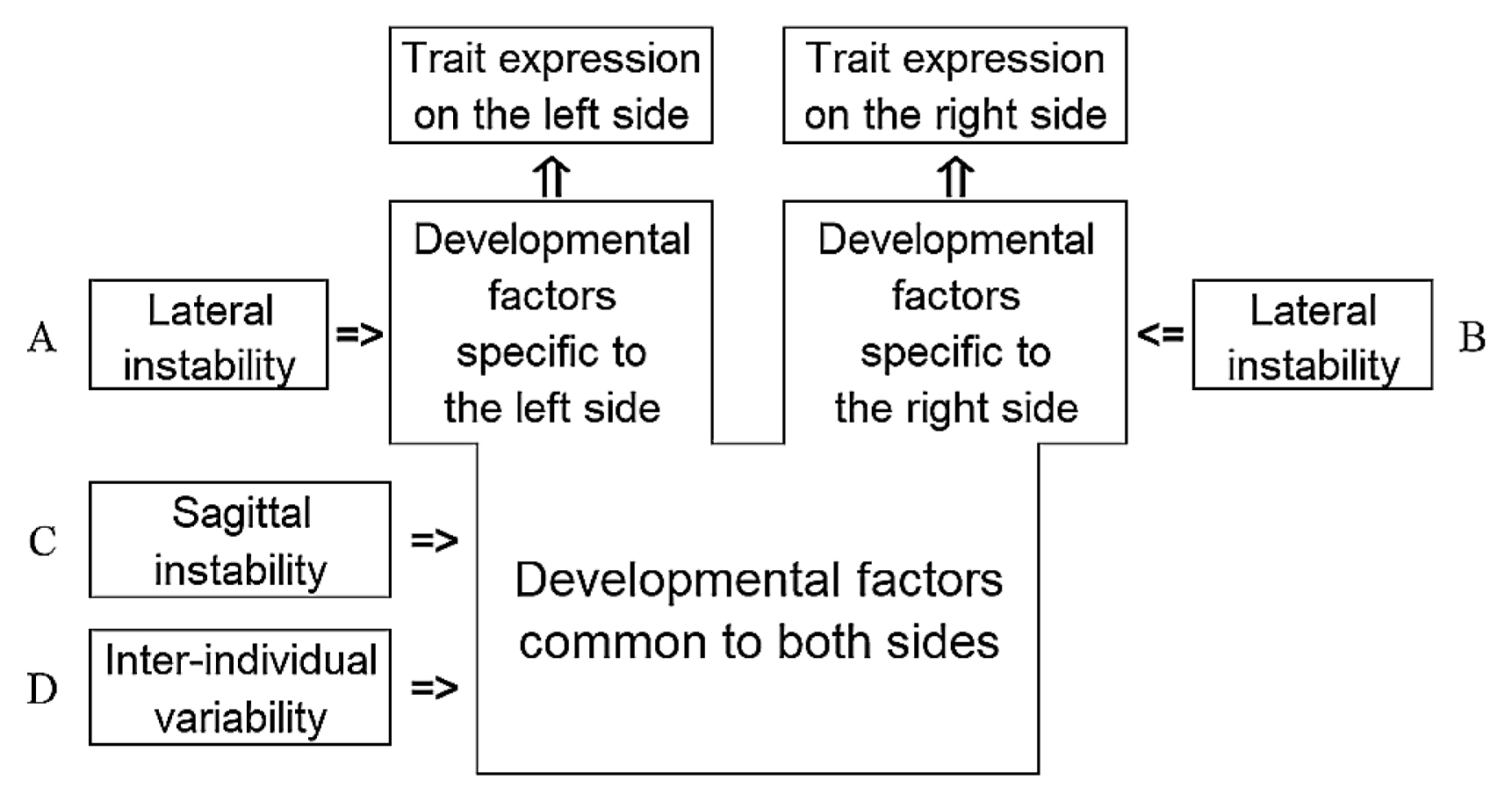
The variability in the development of a trait is explained by the inter-individual variability and within-individual instabilities, i.e. sagittal and lateral instabilities. The sagittal instability creates the fluctuations shared by both sides. The lateral instabilities create mutually independent fluctuations in two sides (Figure 1). These within-individual instabilities are assumed to be constant for all individuals and independent of each other and of the inter-individual variability.
Under this model, the probability of a positive expression for a given individual is identical between sides. Let p be this probability. Then, the probability of asymmetry is equal to 2p(1 − p), and hence never exceeds 50% for any individual. Note that Falconer’s model used by Ossenberg does not include any instability, and hence is not an etiological model when applied to bilateral nonmetric traits. It should be regarded as a convenient model for statistical analyses based on liability.
Constant fluctuation model (CFM)
To examine the goodness of fit of the STM and SGM to data, it is preferable to use a common mathematical framework enabling direct comparison of results. For this, the author uses an extended threshold-type model, called here the ‘constant fluctuation model’ (CFM), which includes both the STM and the SGM. Under the CFM, the expression of a trait (on each side) is explained by a latent variable called ‘liability’ and a constant ‘threshold.’ A positive expression arises when the liability exceeds the threshold. The liability additively reflects various factors and is expressed as the sum of three components: an inter-individual component (IIC) reflecting the genetic and nongenetic factors; a sagittal component (SC) reflecting sagittal instability; and a lateral component (LC) reflecting lateral instability. These components are assumed to be mutually independent. Asymmetry occurs when the interval between the left- and right-side values of the liability contains the threshold. Both the SC and LC are assumed to be normally distributed with zero mean. For simplicity of discussion, it is assumed here that the IIC is genetically determined. Since no preset origin and unit exist for liability, the threshold value is set to be zero and the variance of the LC is set to be 1 hereinafter, unless explicitly specified. Let κ denote the variance of SC. Since the SC is shared by both sides, it would be reasonable to assume that κ is around 0.5. This value is based on the assumption of existence of a general feedback mechanism to control the total variance of phenotypes. Although the feedback will not directly apply to nonmetric traits, the level of instabilities should be controlled by functional traits sharing the same factors of instability as the nonmetric traits.
Under the CFM, the distribution of trait expressions is determined by the distribution of the IIC. To enable statistical analyses based on frequency data, it is assumed that the distribution of the IIC is determined by a limited number of parameters, and at least one of them is determined by the population frequency of the trait when all other parameters are given. The STM is defined as an CFM with a normally distributed IIC determined by two parameters: the mean and the SD. The SGM is defined as an CFM with a binary IIC corresponding to existence/nonexistence of the genotype whose distribution is determined by two parameters: the genotype value and its frequency. Thus, the STM and SGM are contrasting CFMs with equal complexity and degrees of freedom.
The appropriateness of assuming the threshold-type mechanism for the effect of the SC and LC on trait expression is supported by genetic studies. For example, Sucharov et al. (2019) studied heritability of craniofacial traits of zebrafish with variable penetrance and found a liability-threshold nature of penetrance. A study of hearing loss caused by mutations of mitochondrial DNA (Fischel-Ghodsian, 1998) also indicates the threshold model for penetrance of such hearing loss. Although both the studies examined the genetic factors controlling the penetrance, it is reasonable to assume the same mechanism for the effect of the within-individual fluctuations.
General threshold model (GTM)
The general threshold model (GTM) is a family of CFMs whose IIC is distributed with a bell-curved distribution of constant shape, i.e. every parameter of the distribution is constant except for the mean. Accordingly, all the genetic information is carried by the mean of the IIC. This should be the most generalized definition of what are usually considered as threshold models.
The mean of the IIC is estimated from the SCF using the cumulative distribution function of the total liability whose mean is equal to that of the IIC. Apparently, the average of the SCF of two sides is the best estimate for the population value of the SCF. Therefore, the use of the SCF is inevitable for traits conforming to the GTM. Let λ denote the inverse of variance of liability (hence, equal to the proportion of variance of LC to that of liability). Then, the variance of the IIC is equal to 1/λ − 1 − κ, and the population value of the interside correlation of liability is equal to 1 − λ. Unlike the false myth, the inter-side correlation due to the shared variances of IIC and SC is common to all members of the GTM.
Standard threshold model (STM)
The STM is a special case of the GTM with normally distributed IIC. The mean of liability scaled for within-group SD is calculated as the probit of the SCF. The population value of the inter-side correlation of liability is equal to 1 − λ.
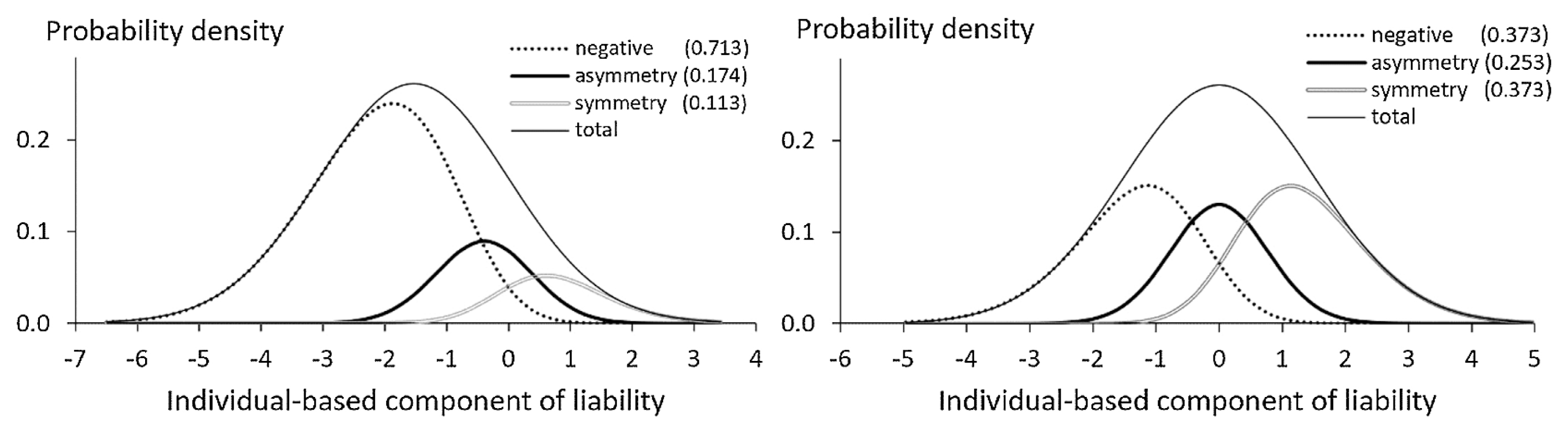
Note that the correspondence between the individual-based value of liability and trait expression is very obscure under the STM. Figure 2 shows the distribution of phenotypes on the individual-based component of liability (IBC) obtained as the sum of the IIC and the SC. Apparently, the mean of liability differs among phenotypes, as Ossenberg (1981) insisted. However, the reproducibility of asymmetry, which is defined as the average probability for the individual with the same value of the IBC exhibiting asymmetry, is much lower than 50%. For example, the values of reproducibility in the left graph of Figure 2 are 86.9% for negative expression, 35.6% for asymmetry, and 55.5% for symmetry, and those in the right graph are 72.5% for both negative expressions and symmetry and 37.7% for asymmetry. The reproducibility based on the IIC is still lower than that based on the IBC. Therefore, the direct examination of ‘heritability of asymmetry’ by McGrath et al. (1984) is unrealistic even if a correct statistical method is used. It would be difficult to understand this using the graphic illustrations in McGrath et al. (1984) and Hallgrímsson et al. (2005).
Under the GTM, the genetic status of a population is represented by the SCF. For population comparison of the SCF to make sense, the distribution curve of the IIC (hence that of total liability too) must be constant across populations. Under the STM, this condition is the constant λ across populations.
Under the SGM, the ICF can be used for population comparison if the penetrance rate is constant across populations, a condition that is equivalent to constancy of the genotype value of the IIC. Although it is usually not possible to directly examine the penetrance rate or the genotype value, the appropriateness of this assumption can be examined by testing the stability of PA across populations; this determines the penetrance rate and the genotype value under the SGM as shown in Table 2.
Table 2
Penetrance rate estimated from the PA under the SGM
| PA |
Magnitude of sagittal instability |
| κ = 0.0 |
κ = 0.25 |
κ = 0.5 |
κ = 1.0 |
κ = 2.0 |
| Penet |
IICa |
Penet |
IICa |
Penet |
IICa |
Penet |
IICa |
Penet |
IICa |
| 0.01 |
1.000 |
2.57 |
1.000 |
2.87 |
1.000 |
3.13 |
0.999 |
3.59 |
0.999 |
4.32 |
| 0.03 |
1.000 |
2.16 |
0.999 |
2.41 |
0.999 |
2.62 |
0.997 |
2.97 |
0.994 |
3.52 |
| 0.05 |
0.999 |
1.95 |
0.998 |
2.16 |
0.997 |
2.34 |
0.994 |
2.64 |
0.988 |
3.09 |
| 0.10 |
0.997 |
1.62 |
0.994 |
1.78 |
0.990 |
1.91 |
0.981 |
2.11 |
0.965 |
2.40 |
| 0.20 |
0.988 |
1.22 |
0.976 |
1.30 |
0.964 |
1.36 |
0.940 |
1.44 |
0.897 |
1.50 |
| 0.30 |
0.969 |
0.93 |
0.945 |
0.95 |
0.921 |
0.96 |
0.876 |
0.93 |
0.797 |
0.80 |
| 0.40 |
0.938 |
0.67 |
0.896 |
0.64 |
0.857 |
0.59 |
0.785 |
0.46 |
0.667 |
0.15 |
| 0.50 |
0.889 |
0.43 |
0.825 |
0.34 |
0.767 |
0.23 |
0.667 |
0.00 |
0.511 |
−0.51 |
| 0.60 |
0.816 |
0.18 |
0.726 |
0.02 |
0.648 |
−0.14 |
0.520 |
−0.49 |
0.341 |
−1.23 |
| 0.70 |
0.710 |
−0.10 |
0.592 |
−0.33 |
0.495 |
−0.57 |
0.350 |
−1.06 |
0.181 |
−2.06 |
| 0.80 |
0.556 |
−0.43 |
0.414 |
−0.76 |
0.311 |
−1.09 |
0.178 |
−1.76 |
0.061 |
−3.10 |
| 0.90 |
0.331 |
−0.91 |
0.196 |
−1.38 |
0.118 |
−1.86 |
0.044 |
−2.80 |
0.006 |
−4.68 |
| 0.95 |
0.181 |
−1.31 |
0.083 |
−1.91 |
0.039 |
−2.51 |
0.009 |
−3.70 |
0.000 |
−6.06 |
| 0.97 |
0.113 |
−1.57 |
0.042 |
−2.26 |
0.016 |
−2.94 |
0.002 |
−4.29 |
0.000 |
−6.98 |
| 0.99 |
0.039 |
−2.06 |
0.009 |
−2.91 |
0.002 |
−3.75 |
0.000 |
−5.42 |
0.000 |
−8.73 |
a genotype value of liability
Ossenberg (1981) used the stability of the formally calculated threshold interval to prove that the negative PA–SCF correlation is an inevitable consequence for threshold traits. This relationship also holds for traits conforming to the STM (Figure 3).
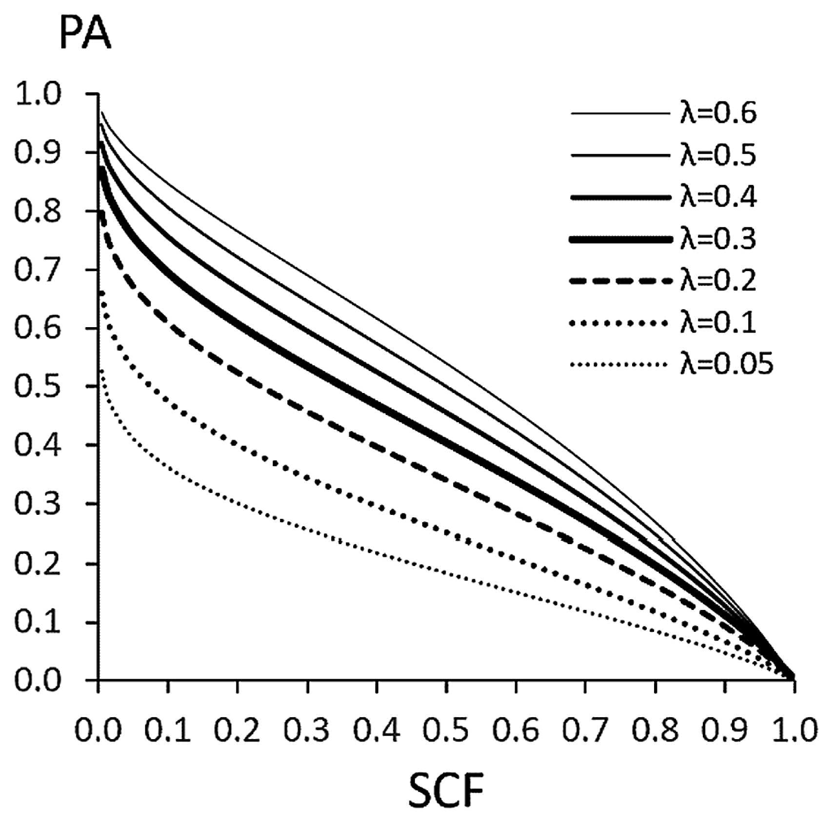
The strategy of Ossenberg’s proof can be adapted to a more general model. As Figure 4 shows, under the GTM with exponentially distributed IBC, both the formally calculated ‘threshold interval’ and the PA are constant. Therefore, a negative PA–SCF correlation arises if the tail decreases more rapidly, i.e. if the distribution is ‘non-heavy-tailed.’ Let us define ‘regular threshold model’ (RTM) as a GTM whose IBC has non-heavy-tailed distribution. Then, the negative PA–SCF correlation is a mathematical consequence of the RTM. Considering that the liability of an actual trait has a finite range of distribution, the RTM covers substantially all the so-called threshold models. Thus, the PA–SCF correlation can be used to distinguish between the RTM and SGM, as Ossenberg (1981) proposed.
Single genotype model (SGM)
The SGM is formulated as a special case of the CFM with a binary IIC. It explains the trait expressions by existence/nonexistence of a genotype and its incomplete penetrance. The term ‘genotype’ is defined here as a latent trait expression determined by a limited number of alleles. The IIC takes the ‘genotype value’ for existence of the genotype and ‘non-genotype value’ for nonexistence of the genotype. If the possibility of a false positive (due to a relatively high non-genotype value) is negligible, both the total penetrance rate and the PA of the genotype are expected to be constant across populations because the genotype value of the IIC is constant across populations. When the penetrance rate is known, the frequency of genotype in a population is estimated as the value of the ICF divided by the penetrance rate.
Relationship between PA and penetrance rate
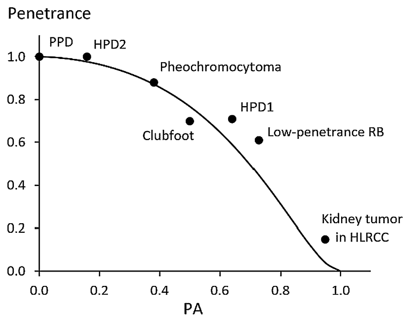
Under the SGM with a known κ, the rate of penetrance is determined by the value of the PA and vice versa (Table 2). Since various congenital anomalies are considered to conform to the SGM, the relationship of their penetrance rates and PA values will serve as strong evidence for the appropriateness of the SGM. Seven cases found in the literature were used to examine this possibility. The value of κ is assumed to be 0.5 for all the cases examined. The maximum likelihood estimation (MLE) method was used to calculate the chi-square values testing the deviation of reported data from the SGM with κ = 0.5 whenever possible. Figure 5 shows a summary of the studies described below.
Gurnett et al. (2008) studied human congenital clubfoot caused by mutation of a specific gene with penetrance considered to be 70% and a rough estimate of 0.50 for the PA. The penetrance rate predicted from the PA = 0.50 equals 77%.
A study of a large pedigree of Chinese with congenital preaxial polydactyly (PPD) by Li et al. (2009) gives another example. The frequency of PPD is estimated to be from 0.05 to 0.2%. They examined the pedigree of 45 individuals including 21 affected individuals and reported 100% penetrance and all the affected individuals had PPD on both sides.
Bourgeois et al. (1998) reported hindlimb polydactyly (HPD) in mice caused by a mutation with penetrance rate 71% and PA = 0.64. The penetrance rate predicted from this PA under the SGM equals 60%. The frequencies they reported were 64 individuals with negative expression, 45 left side only, 56 right side only, and 58 on both sides, which does not significantly deviate from the SGM (χ2 = 4.67, d.f. = 2, P = 0.10).
Chen et al. (2020) also reported HPD in mice caused by another mutation with complete penetrance and PA = 15.8%. The penetrance rate predicted from this PA equals 97.7%. The number of examined individuals is unclear, but seems to be 19 judging from the context. If so, the observed penetrance (19/19) is not statistically different from the expected value (χ2 = 0.88, d.f. = 1, P = 0.35)
A common type of retinoblastoma (RB) affects both eyes with nearly complete penetrance, but a rarer type is known to affect mostly unilaterally with lower penetrance. Although Matsunaga (1978) explained this by the difference of host resistance, Bremner et al. (1997) identified the genetic cause of the low-penetrance RB. They reported 61% for its penetrance and 8/11 for the PA of the affected individuals. The penetrance rate predicted from this value of PA equals 44.8%. The observed PA (0.73) is not statistically significant from the value of the PA (0.63) expected for 61% penetrance (χ2 = 0.47, d.f. = 1, P = 0.49).
Imai et al. (2013) surveyed pheochromocytoma caused by a specific mutation in Japan. The penetrance rate was 25% by 30 years of age, 52% by 50 years of age, and 88% by 77 years of age. They found that 43% (212/493) of patients had developed tumors by the time of survey with PA = 0.38. The penetrance rate predicted from this value of the PA equals 87%. This suggests the possibility of predicting the final penetrance rate from the PA in the early stage of a longitudinal survey.
Kidney tumors in carriers of a mutation causing hereditary leiomyomatosis and renal cell carcinoma syndrome (HLRCC) expected to have the lifetime penetrance of 15% (Menko et al., 2014) and predominantly unilateral occurrence. Merino et al. (2007) reported 36/38 as the PA. The penetrance rate predicted from this PA equals 4% for κ = 0.5. Under the SGM, the PA value corresponding to 15% of penetrance equals 0.883. The observed PA (36/38) is not statistically significant from this value (χ2 = 1.87, d.f. = 1, P = 0.17).
Procedures for analyses of data
The theories presented above suggest the following methods for analyses of bilateral nonmetric traits using actual data. First, the variability of PA is examined to clarify the phenomenon. Second, the PA–SCF correlation is examined for each trait to assess the possibility of applying the STM and SGM. Finally, the goodness of fit of the STM and SGM to the data is examined. These procedures were used for analyses of the data of bilateral nonmetric traits collected by Ossenberg (2013a, b) to test the applicability of the models.
Methods
The data used for analyses were taken from the database of cranial nonmetric traits published on the internet by Ossenberg (2013a, b). The data were divided into samples representing regional populations for each sex (Table 3) in the same way as in Tagaya (2020).
Table 3
Grouping and sample size of the data included in analyses
(Group)
Population |
Sample size |
Composition |
| M |
F |
Total |
| (Africa) |
(195) |
(167) |
(362) |
|
| Khoisan |
24 |
13 |
37 |
San and Khoe speakers |
| North Africa |
48 |
32 |
80 |
Mainly from Kerma site in Sudan |
| Sub-Sahara |
89 |
94 |
183 |
East, West, and South Africans excluding Khoisans |
| US African |
34 |
28 |
62 |
US inhabitants of African origin |
| (Indo-Europe) |
(416) |
(315) |
(731) |
|
| Europe |
344 |
260 |
604 |
Ancient and modern Europeans including British Canadians |
| India |
72 |
55 |
127 |
Housed in University of Alberta |
| (Australia) |
(30) |
(23) |
(53) |
|
| Australia |
30 |
23 |
53 |
Australian Aboriginals including Tasmanians |
| (Jomon-Ainu) |
(204) |
(196) |
(400) |
|
| Jomon |
122 |
133 |
255 |
From Honshu and Hokkaido, including Epi-Jomon |
| Ainu |
82 |
63 |
145 |
Mostly from Hokkaido |
| (NE Asia) |
(534) |
(303) |
(837) |
|
| Japan |
444 |
264 |
708 |
Yayoi, medieval, Edo, and modern Japanese |
| NE Asia |
90 |
39 |
129 |
Manchuria and Mongolia |
| (Circum-Arctic) |
(1342) |
(1418) |
(2760) |
|
| Siberia |
95 |
92 |
187 |
Tungus, Chukchi, Okhotsk, and Yukaghir |
| Aleutian |
210 |
213 |
423 |
Mostly Central and Eastern Aleuts |
| Arctic |
1037 |
1113 |
2150 |
Mainly Inupik and Yupik speakers |
| (America) |
(1066) |
(851) |
(1917) |
|
| America |
1066 |
851 |
1917 |
Athapaskans and non-Arctic Native Americans |
| (Polynesia) |
(73) |
(51) |
(124) |
|
| Polynesia |
73 |
51 |
124 |
Marquesans, New Zealand Maori, and Moriori |
| Total |
3860 |
3324 |
7184 |
|
Table 4 shows the traits included in the analyses. The data of each group consisted of the numbers of individuals with negative (a), asymmetric (b), and symmetric (c) expressions for each trait. The samples with four or fewer sides (5 > b + 2c) were excluded to decrease the effect of sampling errors and avoid an indefinite value of PA.
Table 4
Cranial nonmetric traits included in the analyses
| Code |
Trait |
N of popl. |
sample size |
| m |
f |
m |
f |
| OMB |
occipito-mastoid ossicle |
15 |
14 |
2776 |
2366 |
| AST |
asterionic ossicle |
15 |
15 |
3079 |
2642 |
| PNB |
parietal notch bone |
16 |
15 |
3222 |
2769 |
| POS |
posterior condylar canal absent |
16 |
16 |
3209 |
2745 |
| HYP |
hypoglossal canal bridged or double |
14 |
14 |
3243 |
2805 |
| PCP |
paracondylar process |
14 |
11 |
2660 |
2072 |
| ICC |
intermediate condylar canal |
16 |
15 |
2962 |
2530 |
| SQS |
parietal process of temporal squama |
8 |
7 |
2802 |
2240 |
| MAR |
marginal foramen of tympanic plate |
16 |
13 |
3351 |
2761 |
| TYM |
tympanic dehiscence |
15 |
16 |
3481 |
2984 |
| FSP |
dehiscent wall of foramen spinosum or f. ovale |
15 |
16 |
3188 |
2729 |
| LPF |
foramen in lateral pterygoid plate |
13 |
8 |
2334 |
1679 |
| CIV |
pterygospinous bridge complete (foramen of Civinini) |
10 |
6 |
3030 |
2361 |
| PTB |
pterygobasal spur or bridge |
16 |
16 |
3360 |
2876 |
| CLN |
clinoid bridging |
14 |
11 |
2960 |
2509 |
| SOF |
supraorbital foramen |
16 |
16 |
3526 |
3025 |
| FRG |
frontal groove(s) |
16 |
15 |
3082 |
2561 |
| TRS |
trochlear spur |
13 |
13 |
3208 |
2709 |
| OPT |
accessory optic canal |
9 |
8 |
2549 |
2180 |
| ORB |
orbital suture variant |
13 |
13 |
1854 |
1581 |
| CON |
infraorbital suture variant |
13 |
12 |
1430 |
1365 |
| JAP |
transversozygomatic suture |
14 |
13 |
2624 |
2071 |
| M3U |
upper third molar congenitally absent |
14 |
13 |
2742 |
2182 |
| MEN |
accessory mental foramen |
16 |
13 |
2806 |
2147 |
| MHB |
mylohyoid bridge |
15 |
10 |
2636 |
1987 |
| BUC |
retromolar foramen |
9 |
9 |
2327 |
1937 |
| M3L |
lower third molar congenitally absent |
12 |
13 |
2312 |
1842 |
| TRM |
three-rooted mandibular first molar |
8 |
6 |
1602 |
1215 |
The PA–SCF and PA–ICF correlations among groups were evaluated using the Spearman’s rank order correlation coefficient (ρ coefficient). The value of PA was calculated as b/(b + c). The goodness of fit of the two models, STM and SGM, were examined using chi-square values obtained by the MLE procedure. Each instance of the model is determined by two parameters: values of SCF and λ for the STM, and values of ICF and PA for the SGM, where both λ and PA were assumed to be constant across groups. Thus, the degrees of freedom of the chi-square statistic for goodness of fit are equal to the number of groups minus 1 for both models. Therefore, the chi-square statistic can be directly compared between the two models. The odds ratio (OR) for the likelihood of a trait conforming to the STM relative to the likelihood of conforming to the SGM was calculated from the P-values based on the chi-square statistic. The analyses used Microsoft Excel and VBA programs created by the author.
Results
Correlation between PA and trait frequencies
Table 5 shows the values of PA for the 28 nonmetric traits and the Spearman’s correlation coefficient ρ between the PA and two kinds of trait frequency, SCF and ICF. The PA exhibits a wide variability among groups and traits. The correlation between PA and SCF was negative for all 28 traits, with statistical significance at the 5% level for 22 of them. The correlation of PA with ICF was negative for 27 out of 28 traits, with statistical significance at the 5% level for 12 of them.
Table 5
Spearman’s correlation coefficients between the PA and trait frequencies
| Trait |
N of groups |
Sample size |
Frequency |
PA |
PA-SCF correl. |
PA-ICF correl. |
| SCF |
ICF |
Min |
Max |
Pooled |
ρ |
P |
ρ |
P |
| OMB |
29 |
5142 |
0.16 |
0.25 |
0.50 |
1.00 |
0.70 |
−0.472 |
0.010 ** |
−0.368 |
0.049 * |
| AST |
30 |
5721 |
0.18 |
0.27 |
0.45 |
1.00 |
0.68 |
−0.197 |
0.296 |
−0.020 |
0.915 |
| PNB |
31 |
5991 |
0.21 |
0.32 |
0.25 |
0.85 |
0.67 |
−0.520 |
0.003 ** |
−0.270 |
0.142 |
| POS |
32 |
5954 |
0.21 |
0.33 |
0.44 |
1.00 |
0.74 |
−0.682 |
2E-05 *** |
−0.525 |
0.002 ** |
| HYP |
28 |
6048 |
0.17 |
0.29 |
0.50 |
1.00 |
0.81 |
−0.494 |
0.008 ** |
−0.251 |
0.198 |
| PCP |
25 |
4732 |
0.22 |
0.29 |
0.20 |
0.71 |
0.49 |
−0.318 |
0.122 |
−0.160 |
0.445 |
| ICC |
31 |
5492 |
0.29 |
0.43 |
0.50 |
0.91 |
0.67 |
−0.619 |
2E-04 *** |
−0.432 |
0.015 * |
| SQS |
15 |
5042 |
0.05 |
0.08 |
0.50 |
1.00 |
0.77 |
−0.691 |
0.004 ** |
−0.615 |
0.015 * |
| MAR |
29 |
6112 |
0.16 |
0.22 |
0.25 |
0.88 |
0.57 |
−0.455 |
0.013 * |
− −0.280 |
0.141 |
| TYM |
31 |
6465 |
0.29 |
0.36 |
0.08 |
0.78 |
0.38 |
−0.619 |
2E-04 *** |
−0.461 |
0.009 ** |
| FSP |
31 |
5917 |
0.20 |
0.30 |
0.25 |
0.82 |
0.64 |
−0.447 |
0.012 * |
−0.221 |
0.233 |
| LPF |
21 |
4013 |
0.09 |
0.16 |
0.67 |
1.00 |
0.84 |
−0.661 |
0.001 ** |
−0.522 |
0.015 * |
| CIV |
16 |
5391 |
0.06 |
0.09 |
0.60 |
1.00 |
0.75 |
−0.202 |
0.454 |
−0.152 |
0.575 |
| PTB |
32 |
6236 |
0.16 |
0.24 |
0.32 |
1.00 |
0.64 |
−0.629 |
1E-04 *** |
−0.525 |
0.002 ** |
| CLN |
25 |
5469 |
0.13 |
0.18 |
0.00 |
0.78 |
0.56 |
−0.519 |
0.008 ** |
−0.384 |
0.058 |
| SOF |
32 |
6551 |
0.47 |
0.60 |
0.33 |
0.92 |
0.42 |
−0.806 |
3E-08 *** |
−0.771 |
2E-07 *** |
| FRG |
31 |
5643 |
0.30 |
0.39 |
0.13 |
0.86 |
0.47 |
−0.838 |
4E-09 *** |
−0.770 |
4E-07 *** |
| TRS |
26 |
5917 |
0.06 |
0.09 |
0.43 |
1.00 |
0.67 |
−0.381 |
0.055 |
−0.265 |
0.191 |
| OPT |
17 |
4729 |
0.04 |
0.06 |
0.00 |
0.86 |
0.67 |
−0.485 |
0.049 * |
−0.337 |
0.185 |
| ORB |
26 |
3435 |
0.19 |
0.25 |
0.00 |
0.86 |
0.44 |
−0.683 |
1E-04 *** |
−0.534 |
0.005 ** |
| CON |
25 |
2795 |
0.30 |
0.36 |
0.00 |
0.60 |
0.30 |
−0.442 |
0.027 * |
−0.287 |
0.163 |
| JAP |
27 |
4695 |
0.23 |
0.30 |
0.00 |
0.75 |
0.48 |
−0.561 |
0.002 ** |
−0.474 |
0.013 * |
| M3U |
27 |
4924 |
0.17 |
0.21 |
0.00 |
0.56 |
0.38 |
−0.469 |
0.014 * |
−0.388 |
0.046 * |
| MEN |
29 |
4953 |
0.11 |
0.19 |
0.62 |
1.00 |
0.85 |
−0.453 |
0.014 * |
−0.317 |
0.094 |
| MHB |
25 |
4623 |
0.14 |
0.19 |
0.25 |
0.93 |
0.60 |
−0.521 |
0.008 ** |
−0.374 |
0.065 |
| BUC |
18 |
4264 |
0.07 |
0.10 |
0.14 |
0.83 |
0.66 |
−0.210 |
0.403 |
0.043 |
0.864 |
| M3L |
25 |
4154 |
0.19 |
0.24 |
0.17 |
0.70 |
0.40 |
−0.351 |
0.085 |
−0.209 |
0.317 |
| TRM |
14 |
2817 |
0.18 |
0.22 |
0.15 |
0.67 |
0.36 |
−0.535 |
0.049 * |
−0.484 |
0.079 |
Table 6 shows the goodness of fit of the two models to the data. For the STM, the data of only four traits (AST, FRG, OPT, and BUC) exhibited deviation from values expected from the model with statistical significance at the 2–4% levels. The proportions of variance of lateral component, λ, were distributed from 0.079 (with 95% CI from 0.061 to 0.099 for TRM) to 0.675 (with 95% CI from 0.627 to 0.724 for HYP). This is in accordance with the assumption that κ is around 0.5 because λ is expected to be lower than 2/3 if κ = 0.5.
Table 6
Goodness of fit of the STM and SGM to Ossenberg’s data
| Trait |
STM |
SGM |
Ln(OR) |
| λ |
[95% CI] |
χ2 |
d.f. |
P |
PA |
χ2 |
d.f. |
P |
| OMB |
0.416 |
[.375 .460] |
26.35 |
28 |
0.554 |
0.697 |
35.06 |
28 |
0.168 |
1.82 |
| AST |
0.406 |
[.368 .445] |
47.22 |
29 |
0.018 * |
0.682 |
36.01 |
29 |
0.173 |
−2.45 |
| PNB |
0.424 |
[.388 .461] |
29.33 |
30 |
0.500 |
0.666 |
34.86 |
30 |
0.248 |
1.11 |
| POS |
0.623 |
[.579 .669] |
36.28 |
31 |
0.236 |
0.743 |
94.22 |
31 |
3E-08 *** |
16.26 |
| HYP |
0.675 |
[.627 .724] |
33.22 |
27 |
0.190 |
0.808 |
37.76 |
27 |
0.082 |
0.97 |
| PCP |
0.183 |
[.160 .208] |
26.96 |
24 |
0.306 |
0.487 |
39.52 |
24 |
0.024 * |
2.88 |
| ICC |
0.552 |
[.514 .592] |
39.96 |
30 |
0.106 |
0.673 |
55.42 |
30 |
0.003 ** |
3.61 |
| SQS |
0.359 |
[.296 .429] |
15.19 |
14 |
0.366 |
0.771 |
27.28 |
14 |
0.018 * |
3.46 |
| MAR |
0.242 |
[.215 .272] |
28.96 |
28 |
0.415 |
0.573 |
50.25 |
28 |
0.006 ** |
4.76 |
| TYM |
0.136 |
[.121 .153] |
40.85 |
30 |
0.089 |
0.380 |
80.65 |
30 |
2E-06 *** |
11.03 |
| FSP |
0.374 |
[.341 .410] |
41.30 |
30 |
0.082 |
0.645 |
51.42 |
30 |
0.009 ** |
2.31 |
| LPF |
0.591 |
[.520 .667] |
14.76 |
20 |
0.790 |
0.842 |
21.58 |
20 |
0.364 |
1.88 |
| CIV |
0.324 |
[.272 .381] |
15.61 |
15 |
0.409 |
0.753 |
19.54 |
15 |
0.190 |
1.08 |
| PTB |
0.348 |
[.314 .385] |
37.03 |
31 |
0.211 |
0.641 |
88.57 |
31 |
2E-07 *** |
14.16 |
| CLN |
0.191 |
[.164 .220] |
18.50 |
24 |
0.778 |
0.558 |
21.12 |
24 |
0.632 |
0.72 |
| SOF |
0.337 |
[.311 .364] |
29.75 |
31 |
0.530 |
0.416 |
177.25 |
31 |
2E-22 *** |
50.08 |
| FRG |
0.233 |
[.210 .258] |
48.50 |
30 |
0.018 * |
0.473 |
86.95 |
30 |
2E-07 *** |
11.46 |
| TRS |
0.235 |
[.195 .280] |
24.98 |
25 |
0.463 |
0.673 |
23.08 |
25 |
0.573 |
−0.44 |
| OPT |
0.198 |
[.153 .251] |
26.79 |
16 |
0.044 * |
0.670 |
28.90 |
16 |
0.025* |
0.60 |
| ORB |
0.139 |
[.115 .166] |
27.64 |
25 |
0.325 |
0.437 |
34.30 |
25 |
0.102 |
1.45 |
| CON |
0.079 |
[.064 .096] |
35.63 |
24 |
0.060 |
0.299 |
39.40 |
24 |
0.025 * |
0.91 |
| JAP |
0.207 |
[.181 .235] |
34.15 |
26 |
0.131 |
0.476 |
87.35 |
26 |
1E-08 *** |
16.14 |
| M3U |
0.095 |
[.079 .113] |
32.78 |
26 |
0.169 |
0.378 |
67.64 |
26 |
1E-05 *** |
9.54 |
| MEN |
0.670 |
[.606 .737] |
24.99 |
28 |
0.628 |
0.855 |
25.91 |
28 |
0.578 |
0.21 |
| MHB |
0.252 |
[.218 .289] |
27.49 |
24 |
0.282 |
0.599 |
35.96 |
24 |
0.055 |
1.90 |
| BUC |
0.228 |
[.186 .276] |
31.03 |
17 |
0.020 * |
0.664 |
28.15 |
17 |
0.043 * |
−0.80 |
| M3L |
0.109 |
[.091 .129] |
28.50 |
24 |
0.239 |
0.403 |
35.55 |
24 |
0.061 |
1.58 |
| TRM |
0.079 |
[.061 .099] |
13.86 |
13 |
0.384 |
0.359 |
22.30 |
13 |
0.051 |
2.45 |
For the SGM, the data of 15 out of 28 traits exhibited statistically significant deviation from values expected from the model. The statistical significance was at the 0.1% level for seven traits (POS, TYM, PTB, SOF, FRG, JAP, and M3U), at the 1% level for three traits (ICC, MAR, and FSP), and at the 5% level for five traits (PCP, SQS, OPT, CON, and BUC).
The logarithm of OR was negative only for AST, TRS, and BUC. It was higher than 1 for 20 traits, lower than –1 for one trait (AST), and between –1 and 1 for seven traits (HYP, CLN, TRS, OPT, CON, MEN, and BUC). The negative PA– SCF correlation in these traits except for BUC was statistically significant at the 5% level or close to it (P = 0.055 for TRS). If AST conforms to the SGM, its PA (0.68) indicates 53% penetrance for κ = 0.5.
Discussion
False myths
The review of relevant articles has revealed that the unconditional use of conventional methodology has been justified or encouraged by false myths, including ‘the SGM as natural premise,’ ‘strong inter-side correlations disturb the use of the SCF,’ ‘the model-free nature of the MDD,’ and the ‘unbiased nature of the MMD.’ None of these myths requires any difficult scientific theory to understand its falseness. Such simple illusions could never last for years without noncritical attitudes of our community toward baseless discourses conforming to tradition and notions of the scientific tide. The publication of false results and repeated citations in peer-reviewed journals support this view. It would be impossible to completely prevent similar problems; it is necessary for researchers to be sensitive to the tide of science, and misunderstandings and failures may lead to discoveries. However, it is necessary to pay due attention to the possible consequences of compromising scientific integrity.
Interpretation of heterogeneity of PA
It has been neglected that the proof by Ossenberg (1981) of the negative PA–SCF correlation in threshold traits has decisive importance for the theoretical foundation of studies on nonmetric traits. The heterogeneity of PA among populations has been a theoretical obstacle for genetic interpretation of population comparisons based on nonmetric traits. Although Berry (1968) explained it by genetic stress, Trinkaus (1978) proved that asymmetry is too common to explain it by genetic factors and attributed it to environmental stress. Ossenberg’s proof seems to have been the only solution for this problem, but her proposals were dismissed. As a result, the genetic interpretation of population comparisons based on nonmetric traits with heterogenous PA has lost its legitimacy. A number of studies have been conducted neglecting the deficit of their theoretical basis for over 40 years.
The theory proposed here as an extension of Ossenberg’s theory proved that the heterogeneity of the PA is a normal phenomenon under the RTM. Therefore, the use of asymmetry as an index of environmental stress requires taking into consideration the possibility that the difference in the PA is caused by the difference in trait frequency. Under the RTM, if the stress affects the development of the trait negatively, the value of the PA automatically increases, but it does not mean an increase in developmental instability. Considering the nature of within-individual fluctuations and the results of the present study, it is rather unlikely that higher PA reflects increased instability caused by environmental stress as Trinkaus (1978) considered. Most of the studies of the effect of environmental stress on asymmetry of nonmetric traits so far published lack basic information allowing examination of the PA–SCF correlation.
Clinical utility of PA
Hallgrímsson et al. (2005) explained the tendency of higher values of the PA in rare dysmorphologies by negative PA–ICF correlations under the STM. However, congenital anomalies are very often expressed on both sides regardless of their rarity. According to the theory proposed here, it is not the absolute frequency but the penetrance rate that determines the PA value of the anomaly conforming to the SGM.
Genetic causes have been identified for various rare diseases and anomalies. Since direct estimation of the risk of a genetic cause is difficult for such cases, estimation of penetrance from the PA will be beneficial for clinical purposes. Although Allen (1952) attempted this, the proportion of unilateral penetrance has rarely been reported. The SGM with κ = 0.5 seems to be useful for this purpose. Although κ may vary according to the nature of the anomaly, an unexpectedly low penetrance of a symmetric or low-PA anomaly may indicate existence of unidentified factors inevitable for expression of the anomaly.
Applicability of models and its mathematical consequence
The STM with a constant λ across populations proved to be acceptable for 24 out of 28 traits, while the SGM with constant PA across populations proved to be acceptable for 13 traits. The logarithm of OR indicates that the STM was more favorable than the SGM in 25 out of the 28 traits. Considering these results together with the prevalence of negative PA–SCF correlations, it would be appropriate to consider that most of the nonmetric traits examined here conform to the STM although a very few traits may conform to the SGM. Therefore, the SCF should be more appropriate than the ICF for reflecting possible genetic difference at least for most of the traits examined here. Considering that Hallgrímsson et al. (2005) obtained similar results, it is plausible that the STM, or at least the RTM, applies to most nonmetric traits. Therefore, the use of the SCF as the count method and a liability-based distance measure for population comparison will be the appropriate combination for most of the nonmetric traits.
The ASUDAS explicitly adopts the SGM to justify its use of the ICF (Turner et al., 1991). This is theoretically consistent, but the three dental traits included in the present study (M3U, M3L, and TRM) all showed higher plausibility of conforming to the STM than to the SGM. Therefore, various dental traits may conform to the STM rather than the SGM.
On the other hand, the use of the Mahalanobis distance for nonmetric traits is based on the assumption that all the traits included conform to the STM, but no examination of this seems to have been carried out. Konigsberg (1990) and Konigsberg et al. (1993) used random side selection, which decreased the reliability of results and precluded examination of the etiology of the traits.
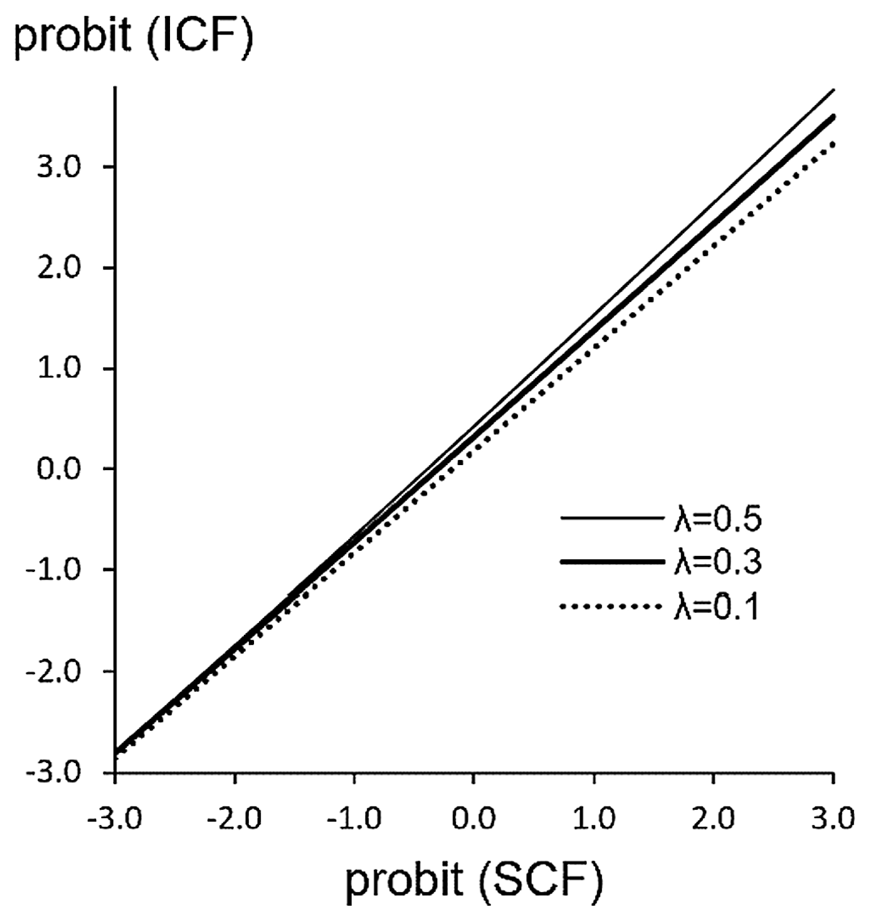
Researchers often use the ICF and the methods based on the STM together. Nikita et al. (2012) used the ICF for the Mahalanobis distance, adopting the side-correlation argument of McGrath et al. (1984). Hanihara (2008) also used the ICF to calculate the threshold values and tetrachoric correlations for the Mahalanobis distance. Godde and Jantz (2017) seem to have used the ICF to calculate the Mahalanobis distance, judging from lack of any description about the definition of the frequency, while they used the data of Hanihara et al. (1998) which reported both the SCF and ICF. The use of the ICF instead of the SCF to calculate the Mahalanobis distance will not substantially affect the resultant overall population relationship because the relationship between the probit of the ICF and that of the SCF (Figure 6) is substantially linear and its slope is only slightly affected by λ. However, the reliability of results significantly decreases. It is recommended to identify the etiological model using the PA–SCF relationship first and then choose the method of analyses appropriate for the identified model.
The reasonable results of analyses and the successful predictions of penetrance rate of congenital dysmorphologies above suggest the usefulness of the theoretical framework proposed. What can be the physical reality of its basic assumption, i.e. the constant within-individual instabilities? The following two studies on cleft lip in twins seem to give a clue. Although the classification system of cleft lip does not allow calculation of the PA, the variable severity and penetrance among several types of cleft lip (Cobourne, 2004) seem to be in accordance with the PA–penetrance relationship under the SGM.
Mansilla et al. (2005) used DNA sequencing to find a mutation responsible for discordance in expressions of cleft lip and palate between monozygotic twins, but found no such mutation in 13 pairs. Takahashi et al. (2018) conducted whole-genome sequencing of a twin pair with mirror cleft lips and found no mutation. These results support the non-genetic nature of the instabilities causing asymmetry. Takahashi et al. stress the possibility of environmental factors being the cause of the discordance of expression between the twin pairs. However, this seems to have resulted from a deterministic view of ‘genetics vs environment.’ The within-individual factors, such as fluctuations of DNA methylation, seem to be more reasonable for explaining their results considering the study of Harris et al. (2019) on the regulation and fluctuations of DNA methylation in the development of honey bees.
Use of sides as individuals
To use sides as if these were individuals to estimate the parameters of distribution of the IIC is statistically acceptable and useful under the STM. Inflation of degrees of freedom due to inter-side correlation (Hallgrímsson et al., 2004) is limited because each side provides independent information about the status of the individual although the information about the population parameters carried by sides is a little less than that carried by the same number of individuals. Simulations under the STM (Table 7) indicate that the standard error (SE) of mean liability based on both sides is about 17–25% less than based on one side for most cases examined. Note that the ratio 0.71 is expected if the same number of other individuals are used. The improvement is larger for traits with higher inter-side correlations of liability (= 1 − λ), unlike the estimation by Green et al. (1979) obtained by assuming that sides are mutually correlated separate traits. Thus, the existence of inter-side correlation does not justify avoiding the use of the SCF and the use of both sides.
Table 7
Ratio of the standard error of estimates for mean liability based on both sides to that based on one side estimated by 10000 simulations
| SCF |
n = 10 |
n = 25 |
n = 100 |
| λ = 0.1 |
λ = 0.3 |
λ = 0.5 |
λ = 0.1 |
λ = 0.3 |
λ = 0.5 |
λ = 0.1 |
λ = 0.3 |
λ = 0.5 |
| 0.05 |
—a |
—a |
—a |
0.86 |
0.89 |
0.89 |
0.73 |
0.74 |
0.76 |
| 0.1 |
0.90 |
0.93 |
0.95 |
0.75 |
0.79 |
0.80 |
0.74 |
0.77 |
0.79 |
| 0.2 |
0.79 |
0.83 |
0.83 |
0.75 |
0.79 |
0.80 |
0.76 |
0.79 |
0.80 |
| 0.3 |
0.76 |
0.80 |
0.81 |
0.76 |
0.80 |
0.81 |
0.77 |
0.79 |
0.81 |
| 0.4 |
0.77 |
0.81 |
0.82 |
0.77 |
0.81 |
0.82 |
0.77 |
0.80 |
0.81 |
| 0.5 |
0.77 |
0.81 |
0.82 |
0.77 |
0.81 |
0.82 |
0.77 |
0.81 |
0.82 |
a Calculation was not performed for cases with SCF less than 1/n because of irrepresentability.
The prevalence of the baseless belief forced Konigsberg (1990) and Konigsberg et al. (1993) to waste a significant portion (probably over 50%) of information in their study using tetrachoric estimation of inter-trait correlations. They used random side selection to treat the bilateral traits as if these were sagittal traits to circumvent possible criticism. However, to regard sides as individuals is efficient, especially in tetrachoric estimations, because the accuracy of the estimates of the correlation of liability between traits considerably improves by regarding four (two parallel and two cross) combinations of sides of the two traits as four independent individuals. The results of simulations (Table 8) indicate that the SE of tetrachoric estimate calculated by regarding the four combinations of sides of two traits as four individuals range from 62% to 79% of those calculated using only one side of the traits. Hence use of the four combinations increases the reliability of the estimate comparable to that obtained using 1.62–2.63 times the number of individuals. The correlation coefficient between IBCs was kept precisely constant in the simulations, and the tetrachoric procedure estimated the correlation for total liability.
Table 8
Standard error of the tetrachoric correlation between traits based on 100 individuals for 1000 simulations with SCF = 0.3 and a constant actual correlation of the IBC
|
λ = 0.1 |
λ = 0.3 |
λ = 0.5 |
| Correlation based on IBC |
0.200 |
0.400 |
0.200 |
0.400 |
0.200 |
0.400 |
| Correlation based on total liabilitya |
0.180 |
0.360 |
0.140 |
0.280 |
0.100 |
0.200 |
| SE of estimate by single combination |
0.144 |
0.135 |
0.156 |
0.152 |
0.169 |
0.166 |
| SE of estimate by four combinations |
0.114 |
0.106 |
0.105 |
0.102 |
0.104 |
0.104 |
| Ratio of SE |
0.79 |
0.78 |
0.67 |
0.67 |
0.62 |
0.63 |
| Ratio of effect sample size |
1.62 |
1.64 |
2.23 |
2.24 |
2.63 |
2.51 |
a calculated by multiplying the correlation based on IBC with 1−λ
The magnitude of estimation errors in Table 8 discourages the use of the Mahalanobis distance. Nikita (2015) cautioned that the Mahalanobis distance with tetrachoric correlations can be seriously affected by sampling errors to produce negative distances. Judging from Table 8, probably 1000 or more individuals will be required to obtain reliable tetrachoric estimates even if the four-combination method is used. The samples of 1082 individuals in Kongsberg (1990), 447 individuals in Konigsberg et al. (1993) and from 250 to 750 individuals in Nikita (2015) seem to be a little too small for reliable estimation of tetrachoric correlations considering that they used random side selection.
Loss of information caused by the use of an inappropriate count method
All the usable genetic information reflected in trait expressions is represented by the ICF under the SGM and by the SCF under the STM. This means that the use of the ICF for traits conforming to the STM loses a certain portion of usable information. Simulations repeated 10000 times for each of various combinations of population values of the SCF and λ under the STM (Table 9) indicate that the SE of angular-transformed frequency increases by from 8% to 29% when the ICF is used instead of the SCF; hence the use of the ICF for traits conforming to the STM means wasting information carried by from 16% to 40% individuals in the samples.
Table 9
Ratios of the standard errors of the angular transformed estimate of the ICF to those of the SCF based on 10000 simulations
| SCF |
n = 10 |
n = 25 |
n = 100 |
| λ = 0.1 |
λ = 0.3 |
λ = 0.5 |
λ = 0.1 |
λ = 0.3 |
λ = 0.5 |
λ = 0.1 |
λ = 0.3 |
λ = 0.5 |
| 0.05 |
—a |
—a |
—a |
1.08 |
1.19 |
1.29 |
1.11 |
1.22 |
1.29 |
| 0.10 |
1.08 |
1.17 |
1.26 |
1.09 |
1.19 |
1.27 |
1.09 |
1.20 |
1.27 |
| 0.20 |
1.08 |
1.17 |
1.25 |
1.08 |
1.17 |
1.25 |
1.09 |
1.18 |
1.25 |
| 0.30 |
1.09 |
1.17 |
1.24 |
1.08 |
1.17 |
1.24 |
1.09 |
1.16 |
1.23 |
| 0.40 |
1.08 |
1.17 |
1.25 |
1.08 |
1.16 |
1.23 |
1.09 |
1.16 |
1.22 |
| 0.50 |
1.09 |
1.16 |
1.21 |
1.10 |
1.17 |
1.26 |
1.08 |
1.16 |
1.23 |
a Calculation was not performed for cases with SCF less than 1/n because of irrepresentability.
Evidence indicates that most of the traits conform to the STM and do not conform to the SGM. Therefore, unconditional use of the ‘golden triad’ is not justifiable. For such traits, MMDs should be replaced with Euclidean distances based on liability because the correlations between traits should be negligible if the MMD has been adopted. The monotonous relationship between the transformation of frequencies between the methods (Figure 7) ensures close similarity of results. The Anscombe-like correction (Tagaya, 2020) may be used for determination of liability corresponding to zero frequency.
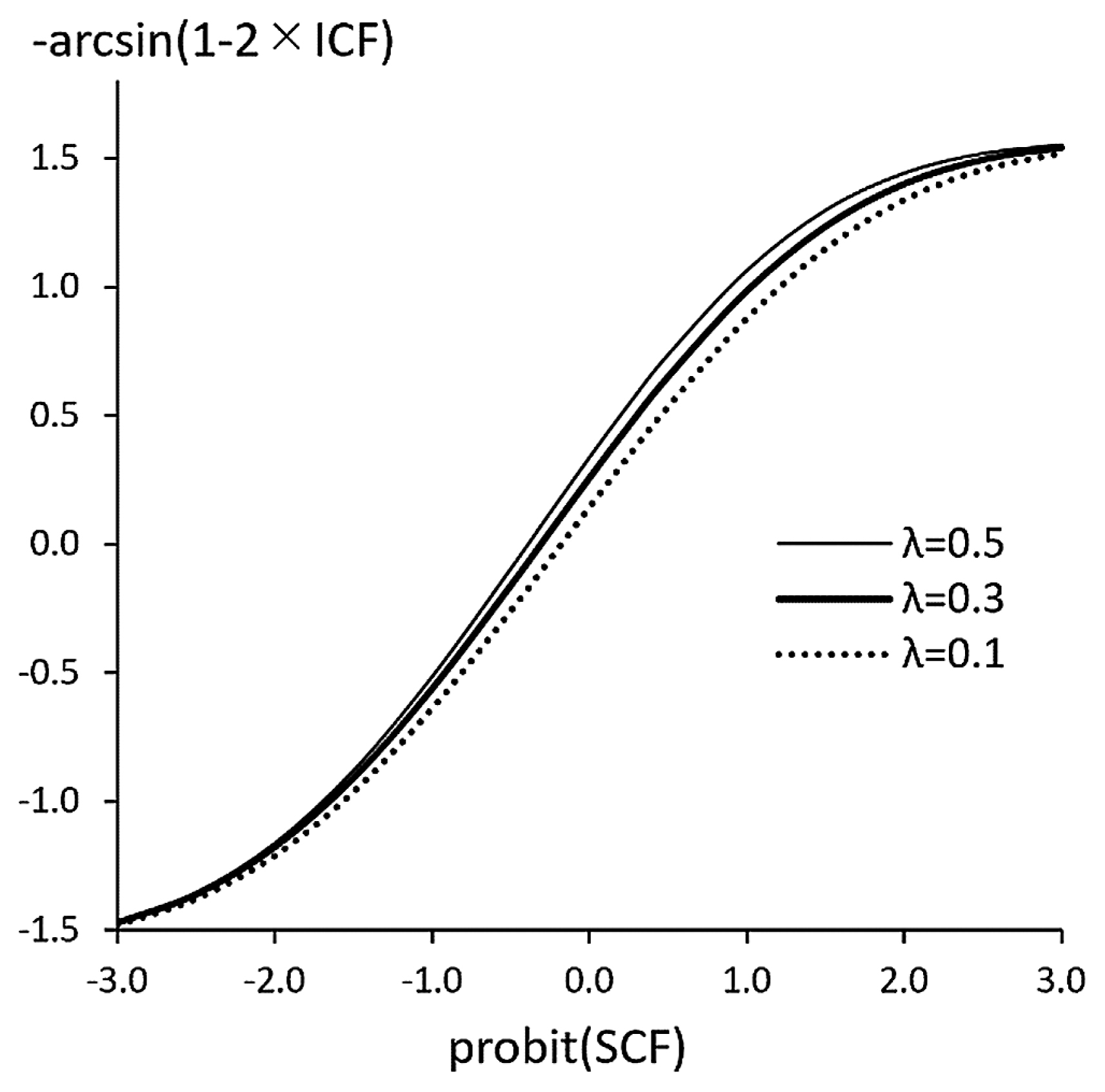
Figure 8 compares the population relationship for males between MMD and Euclidean distance based on the liability of five traits with λ less than 0.5. The overall pattern of the relationship is in fact very close between the two methods. Since the reliability of the frequency statistic used differs between the methods, as already explained, for population relationships differing between the methods, the results based on the means of liability estimated from the SCF should be more reliable.
Rethinking the tradition of reporting count data
In population comparisons based on bilateral nonmetric data, it is inevitable to examine the PA–SCF relationship. Every publication of bilateral nonmetric trait data should include at least two statistics out of the ICF, SCF, and PA to be sufficiently informative. In anthropology, there used to be a reasonable tradition of reporting all the observations that have possible relevance to other researchers. For example, Saito and Ozaki (1936), Ozaki (1938), and Kikuchi (1970) reported frequencies of all the 16 combinations of upper and lower third molar eruption. Ishida and Dodo (1990) reported the frequencies of all the four combinations of bilateral expressions. Hanihara et al. (1998) reported both the ICF and SCF. This tradition was based on wisdom learned from the history that the value of anthropological data increases with time while the results of statistical analyses may lose value after a few decades. However, recent studies tend to report minimum basic statistics or even only the results of analyses. There is no doubt that such a competitive climate helped develop false myths to dismiss inconvenient facts and counterarguments. Ossenberg must have recognized this and chosen to revive her proposals by allowing free access to her raw data.
Conclusions
-
1.
A review of the literature has revealed that the use of the ICF has been justified by false evidence and baseless discourses to dismiss Ossenberg’s arguments for the use of the SCF.
-
2.
The unconditional use of conventional methodology has been justified or encouraged by false myths including ‘the SGM as a natural premise,’ ‘strong inter-side correlations disturbing the use of the SCF,’ ‘the model-free nature of the MDD,’ and ‘the unbiased nature of the MMD.’
-
3.
The author adapted the ideas of Ossenberg to construct a theory based on the assumption of constant within-individual instabilities for generating testable etiological models and exhibited its utility.
-
4.
Most of the nonmetric traits in Ossenberg’s database, including dental traits, are more likely to conform to the STM than to the SGM.
-
5.
The PA can be used to estimate penetrance rate of traits conforming to the SGM.
Acknowledgments
My sincere gratitude is due to the late Dr Nancy Suzanne Ossenberg who made her valuable data open to our academic community. My gratitude is also due to Dr Yukio Dodo who informed me about her passing away and encouraged me to write an article about her contentions. It is not my intention to blame any person for the issues discussed here; all of us are responsible for the problems. I regret that it was not during the lifetime of Dr Ossenberg that I realized the importance of issues involved in her arguments.
References
- Allen G. (1952) The meaning of concordance and discordance in estimation of penetrance and gene frequency. American Journal of Human Genetics, 4: 155–172.
- Berry R.J. (1968) The biology of non-metrical variation in mice and men. In: Brothwell D.R. (ed.), The Skeletal Biology of Earlier Human Populations. Pergamon Press, New York, pp. 103–133.
- Bourgeois P., Bolcato-Bellemin A.L., Danse J.M., Bloch-Zupan A., Yoshiba K., Stoetzel C., and Perrin-Schmitt F. (1998) The variable expressivity and incomplete penetrance of the twist-null heterozygous mouse phenotype resemble those of human Saethre–Chotzen syndrome. Human Molecular Genetics, 7: 945–957.
- Bremner R., Du D.C., Connolly-Wilson M.J., Bridge P., Ahmad K.F., Mostachfi H., Rushlow D., Dunn J.M., and Gallie B.L. (1997) Deletion of RB exons 24 and 25 causes low-penetrance retinoblastoma. American Journal of Human Genetics, 61: 556–570.
- Chen R.Z., Cheng X., Tan Y., Chang T.C., Lv H., and Jia Y. (2020) An ENU-induced mutation in Twist1 transactivation domain causes hindlimb polydactyly with complete penetrance and dominant-negatively impairs E2A-dependent transcription. Scientific Reports, 10: 1–12.
- Cobourne M.T. (2004) The complex genetics of cleft lip and palate. European Journal of Orthodontics, 26: 7–16.
- Donlon D.A. (2000) The value of infracranial nonmetric variation in studies of modern Homo sapiens: an Australian focus. American Journal of Physical Anthropology, 113: 349–368.
- Falconer D.S. (1960) Introduction to Quantitative Genetics. Oliver & Boyd, Edinburgh and London.
- Fischel–Ghodsian N. (1998) Mitochondrial mutations and hearing loss: paradigm for mitochondrial genetics. American Journal of Human Genetics, 62: 15–19.
- Godde K. and Jantz R.L. (2017) Evaluating Nubian population structure from cranial nonmetric traits: gene flow, genetic drift, and population history of the Nubian Nile Valley. Human Biology, 89: 255–279.
- Goldbeter A. (2018) Dissipative structures in biological systems: bistability, oscillations, spatial patterns and waves. Philosophical Transactions of the Royal Society A: Mathematical, Physical and Engineering Sciences, 376: 20170376.
- Green R.F., Suchey J.M., and Gokhale D.V. (1979) The statistical treatment of correlated bilateral traits in the analysis of cranial material. American Journal of Physical Anthropology, 50: 629–634.
- Grewal M. (1962) The rate of genetic divergence of sublines in the C57BL strain of mice. Genetical Research, 3: 226–237.
- Gurnett C.A., Alaee F., Kruse L.M., Desruisseau D.M., Hecht J.T., Wise C.A., Bowcock A.M., and Dobbs M.B. (2008) Asymmetric lower-limb malformations in individuals with homeobox PITX1 gene mutation. American Journal of Human Genetics, 83: 616–622.
- Hallgrímsson B., Donnabháin B.Ó., Walters G.B., Cooper D.M., Guđbjartsson D., and Stefánsson K. (2004) Composition of the founding population of Iceland: biological distance and morphological variation in early historic Atlantic Europe. American Journal of Physical Anthropology, 124: 257–274.
- Hallgrímsson B., Donnabháin B.Ó., Blom D.E., Lozada M.C., and Willmore K.T. (2005) Why are rare traits unilaterally expressed? Trait frequency and unilateral expression for cranial nonmetric traits in humans. American Journal of Physical Anthropology, 128: 14–25.
- Hanihara T. (2008) Morphological variation of major human populations based on nonmetric dental traits. American Journal of Physical Anthropology, 136: 169–182.
- Hanihara T., Ishida H., and Dodo Y. (1998) Os zygomaticum bipartitum: frequency distribution in major human populations. Journal of Anatomy, 192: 539–555.
- Harris E.F. and Sjøvold T. (2004) Calculation of Smith’s mean measure of divergence for intergroup comparisons using nonmetric data. Dental Anthropology Journal, 17: 83–93.
- Harris K.D., Lloyd J.P., Domb K., Zilberman D., and Zemach A. (2019) DNA methylation is maintained with high fidelity in the honey bee germline and exhibits global non-functional fluctuations during somatic development. Epigenetics & Chromatin, 12: 1–18.
- Imai T., Uchino S., Okamoto T., Suzuki S., Kosugi S., Kikumori T., and Sakurai A. (2013) High penetrance of pheochromocytoma in multiple endocrine neoplasia 2 caused by germ line RET codon 634 mutation in Japanese patients. European Journal of Endocrinology, 168: 683–687.
- Irish J.D. (2010) The mean measure of divergence: its utility in model-free and model-bound analyses relative to the Mahalanobis D2 distance for nonmetric traits. American Journal of Human Biology, 22: 378–395.
- Ishida H. and Dodo Y. (1990) Interobserver error in scoring nonmetric cranial traits. Journal of the Anthropological Society of Nippon, 98: 403–409.
- Katayama K. (1981) Genetic study of hypothenar patterns on the palm: estimation of the heritability of liability. Journal of Human Genetics, 26: 279–288.
- Kikuchi S. (1970) Studies on the third molar teeth of men in Self-Defense Forces. National Defense Medical Journal, 17: 73–95 (in Japanese with English summary).
- Konigsberg L.W. (1990) Analysis of prehistoric biological variation under a model of isolation by geographic and temporal distance. Human Biology, 62: 49–70.
- Konigsberg L.W., Kohn L.A., and Cheverud J.M. (1993) Cranial deformation and nonmetric trait variation. American Journal of Physical Anthropology, 90: 35–48.
- Korey K.A. (1980) The incidence of bilateral nonmetric skeletal traits: a reanalysis of sampling procedures. American Journal of Physical Anthropology, 53: 19–23.
- Li H., Wang C.Y., Wang J.X., Wu G.S., Yu P., Yan X.Y., Chen Y.G., Zhao L.H., and Zhang Y.P. (2009) Mutation analysis of a large Chinese pedigree with congenital preaxial polydactyly. European Journal of Human Genetics, 17: 604–610.
- Mansilla M.A., Kimani J., Mitchell L.E., Christensen K., Boomsma D.I., Daack-Hirsch S., Nepomucena B., Wyszynski D.F., Felix T.M., Martin N.G., and Murray J.C. (2005) Discordant MZ twins with cleft lip and palate: a model for identifying genes in complex traits. Twin Research and Human Genetics, 8: 39–46.
- Matsunaga E. (1978) Hereditary retinoblastoma: delayed mutation or host resistance? American Journal of Human Genetics, 30: 406–424.
- McGrath J.W., Cheverud J.M., and Buikstra J.E. (1984) Genetic correlations between sides and heritability of asymmetry for nonmetric traits in rhesus macaques on Cayo Santiago. American Journal of Physical Anthropology, 64: 401–411.
- Menko F.H., Maher E.R., Schmidt L.S., Middelton L.A., Aittomäki K., Tomlinson I., Richard S., and Linehan W.M. (2014) Hereditary leiomyomatosis and renal cell cancer (HLRCC): renal cancer risk, surveillance and treatment. Familial Cancer, 13: 637–644.
- Merino M.J., Torres-Cabala C., Pinto P., and Linehan W.M. (2007) The morphologic spectrum of kidney tumors in hereditary leiomyomatosis and renal cell carcinoma (HLRCC) syndrome. American Journal of Surgical Pathology, 31: 1578–1585.
- Movsesian A.A. (2013) Nonmetric cranial trait variation and population history of medieval East Slavic tribes. American Journal of Physical Anthropology, 152: 495–505.
- Nikita E. (2015) A critical review of the mean measure of divergence and Mahalanobis distances using artificial data and new approaches to the estimation of biodistances employing nonmetric traits. American Journal of Physical Anthropology, 157: 284–294.
- Nikita E., Mattingly D., and Lahr M.M. (2012) Sahara: barrier or corridor? Nonmetric cranial traits and biological affinities of North African Late Holocene populations. American Journal of Physical Anthropology, 147: 280–292.
- Ossenberg N.S. (1981) An argument for the use of total side frequencies of bilateral nonmetric skeletal traits in population distance analysis: the regression of symmetry on incidence. American Journal of Physical Anthropology, 54: 471–479.
- Ossenberg N.S. (1987) Retromolar foramen of the human mandible. American Journal of Physical Anthropology, 73: 119–128.
- Ossenberg N.S. (1992) Native people of the American Northwest: population history from the perspective of skull morphology. In: Akazawa T., Aoki K., and Kimura T. (eds.), The Evolution and Dispersal of Modern Humans in Asia. Hokusen-sha, Tokyo, pp. 493–530.
- Ossenberg N.S. (2013a) Brief communication: Cranial nonmetric trait database on the internet. American Journal of Physical Anthropology, 152: 551–553.
- Ossenberg N.S. (2013b) Cranial nonmetric trait database. Kingston, Ontario, Canada: Nancy, S. Ossenberg [producer]. Queen’s University Library, Data and Government Information Centre [distributor].
- Ossenberg N.S., Dodo Y., Maeda T., and Kawakubo Y. (2006) Ethnogenesis and craniofacial change in Japan from the perspective of nonmetric traits. Anthropological Science, 114: 99–115.
- Ozaki Y. (1938) Mathematical law of distribution of eruption of right and left third molars in the upper and lower jaws. Idengaku Zassi, 14: 247–250 (in Japanese).
- Prigogine I. (1978) Time, structure, and fluctuations. Science, 201: 777–785.
- Relethford J.H. and Lees F.C. (1982) The use of quantitative traits in the study of human population structure. American Journal of Physical Anthropology, 25: 113–132.
- Saito H. and Ozaki Y. (1936) Statistical observation of so-called gingivitis and third molar eruption in Japanese young males. Nihon no Shikai, 202: 1–17 (in Japanese).
- Sato K., Ito Y., Yomo T., and Kaneko K. (2003) On the relation between fluctuation and response in biological systems. Proceedings of the National Academy of Sciences of the USA, 100: 14086–14090.
- Stojanowski C.M., Paul K.S., Seidel A.C., Duncan W.N., and Guatelli-Steinberg D. (2018) Heritability and genetic integration of anterior tooth crown variants in the South Carolina Gullah. American Journal of Physical Anthropology, 167: 124–143.
- Sucharov J., Ray K., Brooks E.P., and Nichols J.T. (2019) Selective breeding modifies mef2ca mutant incomplete penetrance by tuning the opposing notch pathway. PLoS Genetics, 15: e1008507.
- Sutter R.C. and Mertz L. (2004) Nonmetric cranial trait variation and prehistoric biocultural change in the Azapa Valley, Chile. American Journal of Physical Anthropology, 123: 130–145.
- Tagaya A. (2020) Constant sex difference across populations in liability of nonmetric traits. Anthropological Science, 128: 57–70.
- Takahashi M., Hosomichi K., Yamaguchi T., Nagahama R., Yoshida H., Marazita M.L., Weinberg S.M., Makia K., and Tajima A. (2018) Exploration of genetic factors determining cleft side in a pair of monozygotic twins with mirror-image cleft lip and palate using whole-genome sequencing and comparison of craniofacial morphology. Archives of Oral Biology, 96: 33–38.
- Trinkaus E. (1978) Bilateral asymmetry of human skeletal nonmetric traits. American Journal of Physical Anthropology, 49: 315–318.
- Turner C.G., Nichol C.R., and Scott G.R. (1991) Fig University Dental Anthropology System. Advances in Dental Anthropology. Wiley-Liss, New York, pp. 13–31.