1.Introduction
The use of computer-aided drug discovery techniques [1–2] and data analytics [3–5] that allows virtual screening of large databases, structure elaboration, and in silico drug development have accelerated the discovery of new therapeutic agents. In the traditional approach, most bioactive molecules have been discarded at the candidate drug development stage due to problems primarily associated with bioavailability, poor pharmacokinetic profiles, or issues with safety and efficacy [6–8]. Typically, this step is reached at only when substantial amount of resources have already been expended in discovering lead compounds and their derivatives. To avoid this undesirable scenario, additional screens [9–11] that distinguish potentially drug from nondrug compounds have been introduced at the hit-lead discovery stage [12–13] so that only those bioactive hits with druglike characteristics are forwarded for further development.
Several efforts have been exerted to find the chemical features that a compound need to possess for it to be considered a good lead-like or druglike compound [9–11,14–15]. A notable development in this area of medicinal chemistry is the groundbreaking paper of Lipinski on Rule of Five (ROF), which characterizes most orally bioavailable drug candidates [9, 16]. The original ROF specifies critical range of values for four simple physicochemical parameters (i.e. molecular weight, MW ≤ 500; octanol-water partition coefficient, log P ≤ 5; hydrogen-bond donors, HBD ≤ 5; hydrogen-bond acceptors; and HBA ≤ 10) associated with 90% of orally active drugs that have reached the phase II clinical stage. Subsequently, Veber and co-workers established that the optimum number of rotatable bonds (NROT) is 7 and that NROT must not exceed 10 for a compound to display good oral bioavailability [10]. Clark and Pickett also stressed the importance of polar surface area (PSA) in the evaluation of druglikeness and proposed that PSA should not exceed 140 Å2 [11]. Moreover, in ‘fragment-based’ discovery [17–19], the hits identified generally obey a ‘Rule of Three’ (molecular weight, MW ≤ 300; number of hydrogen bond donors, HBD ≤ 3; number of hydrogen bond acceptors, HBA ≤ 3; partition coefficient, ClogP ≤ 3; number of rotatable bonds, NROT ≤ 3; and polar surface area, PSA ≤ 60) [20].
Furthermore, a more ambitious attempt to rapidly distinguish druglike compounds was made by Kubinyi and Sadowski [21] who developed a scoring scheme involving atomic physicochemical parameters [22] that can be used to classify molecules as drug or nondrug. A similar study aimed to distinguish between drugs and nondrugs by predicting the activity spectra for substances (PASS) [23] utilized substructure descriptors called “multilevel neighborhoods of atoms” based on the 2D representation of the molecules [24]. A more recent account also used limited number of molecular descriptors to classify compounds based on assigned probabilities [25].
Aside from the physicochemical properties associated with oral bioavailability [9-11], and the limited structure-derived descriptors used in the pioneering works in this area [21–25], the number of additional chemical descriptors that have been developed has grown [26-28] and the computational tools used to calculate them have become widely available [29]. An enormous number of physicochemical, electrotopological and graph theory-derived molecular descriptors [26–28] are still largely unexplored in virtual high throughput screening of compounds in drug discovery and development. These molecular properties can be quickly calculated from the composition and structure of a compound [30]. A cheminformatics software Dragon® [31], for example, is capable of generating over 4000 molecular descriptors per molecule. The descriptors can be classified as 0D (constitutional properties), 1D (e.g. functional groups, atom centered fragments, information, and other molecular properties), 2D (e.g. topological, molecular walk counts, Burden eigenvalues, eigenvalue based indices, topological charge indices, connectivity, edge adjacency, and 2D autocorrelation), and 3D (charge, Randic molecular profiles, geometry, RDF, 3D-MoRSE, WHIM, and GETAWAY) [32]. We have demonstrated the utility of these molecular descriptors in predicting the activity of different sets of compounds against their corresponding molecular targets [33–35].
The identification of key molecular descriptors that confer druglikeness has been a long-standing goal in drug discovery. ROF, for instance, identified properties that promote oral bioavailability, which is being linked to druglike character of a compound. However, passing the ROF does not guarantee druglikeness [36]. A quick survey of the DrugBank (www.drugbank.ca) will show that TB drugs, antibiotics, and many other drug classes are not in agreement with ROF. The limited scope of ROF [9], the scanty descriptors used in earlier studies to classify molecules as drug or nondrug [21–25], and the scarcity of studies that exploit the intrinsic capacity of diverse molecular descriptors in discriminating drugs from nondrugs have prompted us to cast a wider net in hopes of finding alternative predictors of druglikeness.
As an offshoot of our previous work that employed Discriminant Analysis (DA) [37], this work also examined the two sets of compounds, approved drugs from DrugBank and surrogate nondrugs from the Enamine REAL database of synthetic compounds. The 3D structure of each compound was optimized and the Dragon-type molecular descriptors for each one were calculated. Likewise, the molecular descriptors served as the independent variables while the compound class (i.e. drug/nondrug) was the dependent variable. But, since DA assumes homogeneity of covariances matrices [38] that can however be relaxed on large data sets such as the one used in this study, we thought of considering other classification techniques that would not have such data requisite. Accordingly, we employed Logistic Regression and Random Forest methods in this follow-up study.
2.Methodology
Data collection was done using a personal computer running on Microsoft Windows 7 Professional 64-bit Operating System using a 3.50-GHz Intel Core i7-4770K processor with 8.00-GB random access memory (RAM); and the data management, modeling, and analysis were handled using a machine with MacOS Catalina operating system, 3.1-GHz Dual-Core Intel Core i7 processor, and 16-GB RAM.
The structures of approved drugs were retrieved from the DrugBank database (http://drugbank.ca). The 3D structures of the compounds were generated using the CHARMm force field in BIOVIA Discovery Studio (DS) (
http://3dsbiovia.com) and each structure was saved as structure-data file (.sdf). With the use of Dragon 6 software (
https://chm.kode-solutions.net) over 4000 descriptors were calculated per molecule and the output was organized and cleaned in MS Excel. In the spreadsheet, rows and columns that have at least one NAN (Not A Number) entries and those with invariant values were removed; duplicate compounds, large compounds (MW > 1000), small compounds (MW < 100), and those with metal ions were likewise deleted. Some 25 compounds that were not successfully optimized in DS were also earlier excluded from the data set. Consequently, 1788 drug compounds were left for the analysis.
The structures of nondrug compounds were retrieved from Enamine REAL Collection database (
https://enamine.net). Since the Enamine REAL Compounds database downloaded in 2017 is a huge data set of 22 million compounds, a probability sampling technique was applied to derive a representative sample of nondrug compounds. With the observation that the classes of compounds in this collection were entered in no particular order, albeit a group of variants were entered successively, it was assumed that the list of compounds consist of chunks or clusters similar in terms of general attributes. Each cluster would be a mini-representation of the whole set of compounds. To assemble a good representation of the nondrugs, a three-stage cluster sampling was done. On the first stage, the whole collection of compounds was divided into chunks or clusters of 1 million compounds. These clusters were saved as different files, then a cluster or file (11th) was selected randomly (random.org) from among the 22 files. On the second stage, file 11 was divided into 4000 chunks or clusters consisting of 250 compounds each, and again saved as different files. From these 4000 clusters, 20 clusters were randomly selected and combined as one dataset of 5000 nondrug compounds; and then 3D structures were generated, molecular descriptors calculated, and data organized and cleaned like the drugs data set. On the third stage, 1787 compounds were randomly selected to obtain a nondrugs group of comparable size with the drugs group. Thus, there were a total of 3575 compounds in the working data set on 244 variables. It should be noted, however, that Enamine REAL Compounds database, the nondrugs data source, comprises synthetic compounds that already passed the ROF and Veber filters. But since a data source for nondrug compounds upon which to compare properties of drugs has not yet been established to date, compounds from the database were used as surrogate nondrugs. The choice of Enamine REAL database for this purpose was purely arbitrary, like all the previous studies that attempt to predict or quantify the druglikeness of a molecule wherein their choices had been a matter of preference. And as there is no existing criteria to evaluate a database of compounds qualifying it for a negative set, the only criterion applied in differentiating nondrugs from drugs is the absence of overlap between the two sets of compounds such that a compound not found in the drugs group was labeled nondrug.
A 70-30 split was applied to the data set of 3575 compounds that subsequently generated a training set of 2503 compounds (1252 drugs, 1251 nondrugs) and a test set of 1072 compounds (536 drugs, 536 nondrugs). Data modeling and analyses were done with SPSS Statistics 20.0.0 and RapidMiner Studio 9.7.001 (
https://rapidminer.com) software. Logistic Regression and Random Forest modeling were carried out on the training set with the dependent variable (i.e. drug-nondrug classification) and the 244 independent variables (i.e. molecular descriptors).
Logistic Regression [39-40] determines a logistic or logit function (log-odds) to model a categorical dependent variable. This has been applied in various disciplines including mostly medical fields [41–42], social sciences [43], engineering [44], marketing [45], and drug discovery [46–47]. Logistic modeling is a suitable statistical and machine learning technique for classification giving the means for the identification of the determining predictors.
Random Forest (RF) is a machine learning algorithm that is used for classification and regression. As a classifier, it uses an ensemble of decision trees that output the mode of the results (classification) from the trees. A decision tree (DT) is a flowchart resembling a tree showing the process of arriving at an output of the target variable through the values of the features. The chart starts at a root node, then by the branches it reaches the internal nodes, up till the leaf nodes. The root node corresponds to the feature that has the most influence upon the target output, the internal nodes are the other features relevant for the target variable, the branches hold the feature values, and the leaf nodes carry the target output. The features generally characterize the instances in relation to the target variable. A trained DT classifies new instances by tracing their paths from the root node to a leaf node, and this process resembles following a set of decision rules. Thus, decision tree algorithm creates a model that predicts the value for the target variable gathering simple decisions from the data features. The predictive performance of a random forest depends on both the strengths of the individual trees and on the correlation between the trees. Thus, aggregating the results of a multitude of trees trained by modified DT learning algorithm, taking only a random sample of features at each node, results in a robust RF model. In effect, RF combine all the information found in the forest making it more effective in predicting outcomes compared to single decision trees [48]. RF is now one of the most popular machine learning techniques and has been applied in data mining for computational biology [49–50] and medicine [51–52].
DT learning uses some criteria, such as Information Gain and Gini Index, that determine the best features on which to build a tree and cutoff values to split the nodes. Information gain is the reduction in entropy after splitting a node. Entropy is a measure of disorder of the target outputs in the nodes, in which higher values mean greater disorder (impure nodes) and lower values indicate purer nodes. Gini Index is a measure of inequality between the distributions of the target outputs. Like Entropy, lower values of Gini Index indicate purer nodes, and thus the feature that splits a node resulting in a smaller Gini Index or lower Entropy is chosen. Information Gain Ratio is another criterion used in the selection of features taking into account the number and size of branches thereby reducing the bias towards those features with multiple values. And being a classifier, Accuracy, is also used to evaluate the predictive performance of a DT model. Hyperparameters are also considered for speed and quality of the DT learning process, such as the number of predictors to be sampled (mtry) and considered to split a node, and the number of trees (ntree) to be grown in the forest.
3.Results and Discussion
There are several approaches in determining the druglikeness of a compound. The most popular is the Lipinski rule of five (ROF) [9] that is based on certain structural features of the molecule (e.g. count of H-bond acceptors and H-bond donors) along with molecular weight and log P. While ROF and its successors [10,11] have the advantage of having features that require only simple counting and measurement, the rule does not necessarily point to druglikeness for such features were examined only for their association with oral bioavailability. Moreover, rule-based methods essentially use equal weights for all the parameters and entail sharp boundaries that lead to different classifications for highly similar molecules. These apparent limitations are overcome with the use of prediction models that do not only identify the crucial features but also provides more thorough quantitative appraisal for how druglike a compound is. For instance, the quantitative estimate of druglikeness (QED) developed recently by Bickerton [53] exhibits a continuous spectrum from the most druglike compounds to the least druglike ones. Unlike the rule-based classifiers that are prone to misclassification due to abrupt cut-offs, the structurally similar compounds will have comparable QED scores and consequently will have most likely the same predicted drug classification. Notwithstanding this appealing refinement, QED has also been defined mostly by only the traditional descriptors in ROF and its extensions, and need to determine for each class of therapeutics the adjustable weighting factors for the features. The proliferation of molecular descriptors in recent years provides great advantage of being able to consider more features that will be utilized in determining druglikeness. On top of that, the DrugBank database contains not only oral drugs but also those that are administered through other routes, paving the way for the discovery of descriptors that dispense druglikeness intrinsic to a molecule, and not just oral bioavailability.
3.1 Multiple Logistic Regression
The dependent variable in this study is called ‘Compound Class’ with categories ‘Drug’ and ‘Nondrug’ and hence the binary logistic model was used with the Dragon-type molecular descriptors as predictors. Logistic Regression was first implemented on the original set of 244 variables using the default setting of the software. At this instance, 13 descriptors (nBO, nH, nHet, nCIC, Rbrid, Qindex, BBI, SNar, Psi_e_A, MPC01, X0, X1, and TIC0) were excluded for having strong collinearity with the other variables in the set exceeding a correlation coefficient of 0.98. With 231 predictors, Model 1 (Table 1) was constructed with a prediction accuracy of 93.00%, that is, in the test set of 1072 compounds it correctly classified 997 and misclassified only 75 compounds. For the class recall of the model, the sensitivity was 91.60% (out of the 536 drugs it misclassified only 45 as nondrugs) and specificity was 94.40% (out of the 536 nondrugs it misclassified only 30 as drugs). As regards precision, the positive prediction value was 94.24% (only 30 out of 521 predicted drugs are actually nondrugs) and the negative prediction value was 91.83% (only 45 of the 551 predicted nondrugs are actually drugs).
Table 1. Confusion Matrix of Model 1 (LogR Model on Compound Class with 231 Dragon-type Descriptors)

One of the most popular evaluation tools for classification methods is the receiver operator characteristic curve or ROC curve. It is the true positive rate or TPR (sensitivity) as a function of false positive rate or FPR also called fall-out (i.e. 1-specificity). ROC is also known as relative operating characteristic curve as it depicts relative trade-offs between two operating characteristics, TPR and FPR, as the threshold values are varied. It displays the summary of all the corresponding confusion matrices produced by a classification method at different discrimination threshold settings [54–55] so that a point in the curve represents particular instance of a confusion matrix. Perfect classification occurs at point (0,1) where the prediction method yields 100% for both sensitivity and specificity. The diagonal line from point (0,0) to point (1,1) is so-called line of no discrimination that is much the same as random guesses. Curves above the diagonal line represent good classification and the closer an ROC curve is to the top left corner the better, such curves have higher values for both sensitivity and specificity. Compound classification by Model 1 is highly satisfactory with the optimal threshold of the model presenting high values for both sensitivity and specificity (Figure 1).

The area under the curve (AUC) of the ROC curve (or AUC-ROC) is another performance evaluation tool that indicates how much a model is able to separate between the categories of the dependent variable. When AUC equals 1, it means that the method perfectly distinguishes between the two classes so that an excellent model would have an AUC close to 1. An AUC near 0.5 means that the model is not able to differentiate the classes and a value near 0 implies that the classification method reverses its prediction [56]. Model 1 has an AUC of 0.976 conveying that it can almost perfectly distinguish drugs from nondrugs. Model 1 with 231 descriptors on 2503 compounds in the training set satisfies the ‘rule of ten’ (i.e. 10 compounds per descriptor) in Logistic Regression [57].
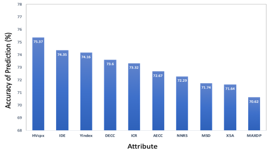
Nevertheless, the major goal of this work was to identify the key structure-derived Dragon-type molecular descriptors that confer druglikeness. Thus, a feature selection process is necessary to generate a model with a good prediction performance while constituting only the most important chemical features. With the 231 descriptors, 1-variable logit modeling was implemented using each of those descriptors. Ten of the resulting single-predictor logit models exhibited at least 70% prediction accuracy (Figure 2). The featured descriptors were HVcpx, IDE, Yindex, DECC, ICR, AECC, NNRS, MSD, X5A, and MAXDP. The two-tailed t-tests done on these variables at 5% level of significance showed significantly different means between drugs and nondrugs. As the best among them, HVcpx singlehandedly distinguishes drugs from nondrugs with 75% accuracy. This result had been consistent with our previous study that employed Discriminant Analysis where the best 2-variable discriminant function also included the descriptor HVcpx, which alone correctly classified 72% of the compounds [37].
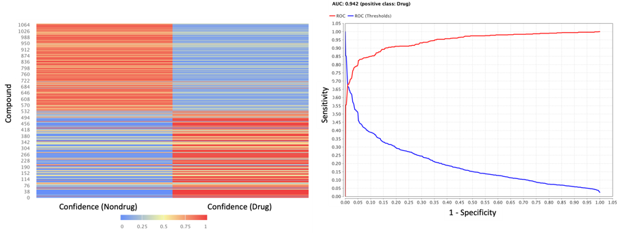
However, with only 75% prediction accuracy, compounds classification was not well resolved yet. Instinctively, the top ten descriptors were put together in a single 10-predictor logit model (Model 2). As a matter of course, this resulted in a raised prediction accuracy of 87.5% and AUC of 0.94 (Table 2). Model 2 adequately separates drugs from nondrugs with high values for both sensitivity and specificity and low classification errors such as false negative rate and false positive rate (Figure 3). The ROC curve likewise presents Model 2 with optimal point on the top left corner near point (0,1) indicating satisfactory classification performance.
Table 2. Prediction Performance of LogR Models on Drug Class
| Model |
LogR Equation |
P-value |
Nagelkerke R Square (%) |
Prediction Accuracy* (%) |
Sensitivity (%) |
Specificity (%) |
AUC |
| 1 |
P = -4.858 MW + 11.611 AMW - … - 53.341 SpPosA_A - 1775a
|
- |
- |
93.0 |
91.6 |
94.4 |
0.98 |
| 2 |
P = -19.003 IDE - 12.468 HVcpx - 64.410 X5A - 2.771 NNRS - 0.243 MAXDP - 0.385 DECC + 4.047 Yindex + 4.784 ICR + 0.810 AECC + 6.152 MSD + 53.654b
|
<0.001 |
56.9 |
87.5 |
80.0 |
95.0 |
0.94 |
| 3 |
P = -0.012 MW + 0.812 AMW + 3.966 RBF - 0.675 nN - 0.061 C% - 2.848 PJI2 + 0.000 Wap + 0.022 MAXDN - 0.496 SRW05 - 5.444 SIC1 + 6.220c
|
<0.001 |
52.6 |
82.3 |
74.2 |
90.3 |
0.88 |
| 4 |
P = -11.87 HVcpx + 0.41 MDDD - 3.42 NNRS + 8.98 X2A - 0.57 SRW05 + 31.09
|
<0.001 |
62.9 |
89.0 |
83.2 |
94.8 |
0.95 |
P = probability that a compound is a drug, * test set (N = 1072), awith 231 predictors (P-value and r2 calculation failed due to multicollinearity), bwith 10 topmost predictors, cwith 10 weakly correlated predictors.
Nonetheless, the correlation matrix was re-examined for these 10 predictors in Model 2 and it revealed 6 highly correlated (r > 0.9) descriptors indicating the presence of multicollinearity and accordingly violating the assumption of independence of variables for the logistic model [58]. To resolve this, the default value set for the correlation coefficient was changed to 0.4 so that variables which are at least moderately correlated are excluded from the analysis [59]. Then another Logistic Regression was carried out on the original set of 244 predictors, and this new setting left only 13 variables for the model. The accuracy of the resulting model was already lower by about 4 percentage points than the previous 10-variable model. For straightforward comparison with the previous 10-variable model, the number of variables in this model was further reduced to 10 using the forward stepping method of feature selection [37]. With this technique, 1-variable logit models were generated in the first round. The descriptor that gave the highest prediction accuracy was carried over to the second round involving 2-variable logit models, that is, the best predictor in round 1 was paired with each and every predictor left in the set. Then the best pair of predictors in round 2 was forwarded to the third round to generate 3-variable models. This procedure was iterated until the best 10-predictor logit model or Model 3 was obtained consisting of only weakly correlated descriptors namely, MAXDN, nN, Wap, MW, AMW, SRW05, SIC1, PJI2, RBF, and C%, according to the order of which they entered into the model. Compared to Model 2 with also 10 predictors but some with strong correlation, this Model 3 had lower values for both predictive accuracy (82.3% vs 87.5%) and AUC (0.88 vs 0.94).
It would seem that some of the descriptors that were excluded due to the stringent requirement on multicollinearity contain information valuable to explain druglikeness. Hence, the correlation coefficient was reset at default value so that only variables that have very strong correlation would be eliminated in the process. Then another feature selection by forward stepping method was done on the 244 variables. HVcpx, the best single variable classifier (Figure 2), was paired with every variable in the set creating 230 two-variable logit models. The best model in this round consisted of the combination of HVcpx and MDDD that displayed a prediction accuracy of 85.4% and AUC of 0.91. This duo is exactly the same pair that constituted the best model in a similar study that employed Linear Discriminant Analysis (LDA) [50]. The predictive performance of this 2-variable model was even higher than Model 3 (Accuracy: 85.4% vs 82.3%, AUC: 0.91 vs 0.88) that included 10 weakly correlated descriptors. The inclusion of NNRS as a third variable enhanced the performance of the model (86.7% accuracy), and with two more variables [X2A and SRW05] into the model the prediction accuracy furthermore increased to 89.0% (Figure 4). Every predictor added to the model increased the confidence of correctly classifying compounds and decreased the probability of misclassification.

The resulting 5-predictor logit model (Model 4) correctly classified 446 of the 536 drugs (i.e. sensitivity was 83.2%) and 508 of the 536 nondrugs (i.e. specificity was 94.8%). Its AUC (Figure 5) further indicated very satisfactory performance correctly classifying 95% of compounds. The addition of the next most influential variable, ON0V, contributed only additional 0.66 percentage point to the prediction accuracy thus further addition of descriptors into the model was no longer pursued. The Nagelkerke R square shows that Model 4 can better predict drug class compared to the two ten-variable models. Except for HVcpx and MDDD which were moderately correlated ( r = 0.78), the rest of the pairs of descriptors in Model 4 were not strongly correlated (r < 0.4) [59].

The most influential descriptor HVcpx is an information index called graph vertex complexity index [60–61]. Model 4 implies that a small value for HVcpx renders a molecule to be more druglike or that a more complex molecule is more likely a drug. The second important descriptor MDDD (mean distance degree deviation or ) is the sum of the differences between the vertex distance degree (i) and the mean vertex distance degree (
σ
¯
), where i is sum of the topological distances or distances of all the other atoms j to atom i (dij). Terminal vertices are observed to have high values of vertex distance degree compared to central vertices. The vertex distance degree is small if the vertex is near a branching site compared to a terminal vertex that is far away from it [28]. The model shows that large values of MDDD are associated with druglikeness, thus, a molecule with distant peripheral groups tend to be a drug. The third most influential variable, NNRS, is a ring descriptor that stands for normalized number of ring systems [27]. A smaller NNRS value favors druglikeness. The ring portions in the molecule provide structural rigidity, which can be useful for anchorage or precise disposition of functional groups during interaction with a biological target. However, the model conveys that smaller NNRS is needed for a molecule to be druglike. The fourth and fifth variables, X2A (average connectivity index of order 2) and SRW05 (self-returning walk count of order 5), are connectivity and walk count indices, respectively [27]. Larger values of X2A and smaller values of SRW05 increase the probability of druglikeness. In general, these descriptors encode the structural complexity of a molecule. Incidentally, the MW in known classifiers are strongly correlated with MDDD (r = 0.89) and HVcpx (r = 0.71). In addition, the normalized number of ring systems (NNRS), although absent in ROF, is related to the number of aromatic rings (AROM) in Bickerton’s QED [53].
3.2 Random Forest
In this work, each tree was grown using 67% of the instances randomly chosen from the training set. The remaining 33% so-called out-of-bag (OOB) samples were utilized to calculate the unbiased prediction error (OOBerror) that was used to evaluate the model accuracy during training. The behavior of the OOBerror as a function of the number of trees, ntree, (Figure 6) was observed for each of the four criteria of feature selection and model performance namely, Gini Index, Information Gain, Gain Ratio, and Accuracy. This in turn became the basis for the determination of the number of decision trees that should be grown in the forest. The OOBerror settled at a constant minimum starting at around 90 trees for all the four criteria. In fact, there were no remarkable changes in the OOBerror values when the number of trees was increased up to 1000 (not shown). Therefore, ntree=100 is just fitting and so this value for the number of trees was used in subsequent analyses. Information Gain and Gini Index showed comparable OOBerrors that are remarkably lower than those of Gain Ratio and Accuracy. Accordingly, either Information Gain or Gini Index was used in the prediction and validation steps.

The suitable maximal depth of each tree was also determined by plotting the OOBerror against the depth of each decision tree (figure not shown). The OOBerror curve was stabilized starting at depth of 7 for the criterion Accuracy, and at 20 for the other criteria. Using the optimal parameters (ntree = 100, depth of tree = 20) with Gini Index as the selection criterion and confidence vote as the voting strategy, an RF model involving the 244 features (Model 5) was applied to the test set. With prediction accuracy of 94.2% and AUC of 0.982 (Table 3), this model performed better than the 231-predictor logit model (Model 1). Based on the attribute weights shown by the model, the 10 most influential descriptors are simply constitutional indices: N% (percentage of N atoms), AMW or average molecular weight (MW/nAT, where nAT is the number of atoms), MW (molecular weight, the sum of atomic weights), Si (sum of first ionization potentials), Mv (mean atomic van der Waals volume), Mp (mean atomic polarizability), Se (sum of atomic Sanderson electronegativities), Mi (mean first ionization potential), Sp (sum of atomic polarizabilities), and nBT (number of bonds)[29].
However, when RF was implemented on only the five predictors in Model 4, the accuracy of the corresponding model (Model 6) was decreased to 86.7%, which is 2.3 percentage points lower than that of Model 4, albeit AUC remained high at 0.940. This slightly inferior outcome was the apparent result of having very few variables to create a forest. With only subsets of already small set of variables on which to create trees, only very few tiny trees would have been built that resulted in an information deficient random forest. More features would have been needed in order to build a powerful random forest. As a matter of fact, when another RF was carried out on the 10 predictors in Model 2, the resulting model (Model 7) performed much better (Accuracy = 89.9% vs 87.5 and AUC = 0.96 vs 0.94). Like Model 5 that performed better than its corresponding logit Model 3, Model 7 as well performed better than its 10-variable logit Model 2 counterpart. Most interestingly, the random forest Model 8 propagated by the 10 weakly correlated predictors performed even much better (Figure 7) than the corresponding logit Model 3 (Accuracy = 92.5% vs 82.3% and AUC = 0.97 vs 0.88). This remarkable performance of Model 8 with 10 predictors was only 1 and 2 percentage points shy of the accuracy of logit Model 1 and random forest Model 5, respectively, that consisted of more than 200 predictors!
Table 3.Prediction Performance of RF Models on Drug Class
| Model |
Input Variables in Random Forest Model
(in order of decreasing attribute weight)
|
Prediction Accuracy (%) |
Sensitivity (%) |
Specificity (%) |
AUC |
| 5 |
N% > AMW > MW > Si > Mv > Mp > Se > Mi > Sp > nBT >>> IDMTa
|
94.2 |
91.4 |
97.0 |
0.982 |
| 6 |
MDDD > HVcpx > X2A > NNRS > SRW05
|
86.7 |
83.0 |
90.3 |
0.941 |
| 7 |
MSD > AECC > DECC > MAXDP > ICR > Yindex > X5A > NNRS > IDE > HVcpxb
|
89.9 |
86.2 |
93.7 |
0.962 |
| 8 |
MW > AMW > RBF > C% > MAXDN > Wap > SIC1 > nN > PJI2 > SRW05c
|
92.5 |
90.1 |
95.0 |
0.970 |
awith 231 descriptors, bwith 10 topmost descriptors, cwith weakly correlated descriptors (r < 0.4).
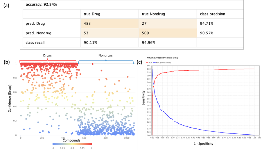
Each of the ten weakly correlated descriptors in Model 8 (Table 4) carried unique and vital information required in producing a diversified forest that yielded more accurate predictions. Half of the descriptors in Model 8 (and Model 3) were constitutional indices: MW (molecular weight), AMW (average molecular weight), RBF (rotatable bond fraction), C% (percentage Carbon), and nN (number of nitrogen atoms). On the other hand, MAXDN (maximal electrotopological negative variation), Wap (all-path Wiener index), and PJI2 (2D Petitjean shape index) are topological indices; SIC1 (structural information content index, neighborhood symmetry of 1 order) is an information index; and SRW05 (self-returning walk count of order 5) is a walk and path count index [27]. The model correctly classified 90% of the drugs and 95% of the nondrugs and misclassified no greater than 10% of the drugs.
Table 4. Correlation of Descriptors in Model 8 (RF Model on Drug Class)

In this endeavor, the interpretation of the descriptors poses a challenge as most Dragon-type descriptors have extremely difficult chemical interpretations, and this makes their application in drug design quite daunting. Fortunately, for Model 5 and Model 8, the descriptors with the most information for druglikeness are largely constitutional indices that have straightforward chemical interpretations. Model 8 had a false negative rate of 9.89%, that is, it misclassified 53 out of 536 true drugs. Notably, a sizeable number (20 or 38%) of the misclassified drugs act on receptors associated with the central nervous system including the drugs for schizophrenia (Remoxipride, Sulpiride, and Olanzapine), and depression or anxiety (S-Adenosylmethionine, Fluvoxamine, Droperidol, Buspirone, Trazodone, and Flurazepam). The rest are antihypertensive drugs Isradipine, Nisoldipine, Prazosin, Brimonidine, Carteolol, Labetalol, Phentolamine, and Furosemide, and some commonly known drugs shown in Table 5. The ten descriptors of Model 8 (Table 3) are arranged in decreasing order of attribute weight. MW has the largest attribute weight with the drugs group having larger molecular weights. Of the 53 false negatives, 34 or 64% have molecular weights smaller than the lower bound of the 95% CI for the drugs group. Misclassifications result from having values that are not typical for the particular drug group, like values outside the 95% CI, on at least one of these 10 descriptors. The values on these features of a given molecule contribute to the probability that such would be classified as drug or nondrug. Although an optimal threshold value such as that determined by the Youden index [62] could afford an improved prediction performance, the cutoff value applied here was fixed at 0.5 simply due to its straightforwardness. Thus, the drugs with calculated probabilities below 0.5 were classified as nondrugs and comprise the false negatives (FN).
Table 5. Commonly Known Drugs Misclassified as Nondrugs by Model 8
In all of these, it should be noted that the nondrug compounds used in this study are rather surrogate nondrugs, which were taken from Enamine REAL Collection database that comply with ROF and Veber criteria for oral bioavailability. Consequently, the crucial descriptors unveiled in these study are those that distinguish approved drugs of all sorts (i.e. oral drugs and those that are administered through other routes) from nondrugs, which are represented by Enamine REAL compounds.
4.Conclusion
Logistic Regression and Random Forest models were generated using 244 variables from the original number of 4000 Dragon-type molecular descriptors derived from 3575 compounds. With the main objective of identifying alternative predictors for druglikeness, the models were trained on 70% of the samples (2503 compounds) and tested on the remaining portion of the samples (30% or 1072 compounds).
Based on the best LogR model in this study with prediction accuracy of 89.0%, the five most influential descriptors for druglikeness arranged in decreasing order of importance are: an information index HVcpx called graph vertex complexity index, topological index MDDD or mean distance degree deviation, a ring descriptor NNRS that stands for normalized number of ring systems, X2A or average connectivity index of order 2, and walk and path count SRW05. In general, a more structurally complex molecule (i.e. smaller HVcpx), with more distant peripheral groups (i.e. larger MDDD, X2A), fewer rings (i.e. smaller NNRS), and less branching around odd-membered rings (i.e. smaller SRW05) tends to be a drug. Interestingly, HVcpx, MDDD, and NNRS are correlated with some descriptors in well-known classifiers.
On the other hand, the best RF model with prediction accuracy of 92.5% identifies the following 10 descriptors in order of decreasing attribute weights: molecular weight, MW; average molecular weight, AMW; rotatable bond fraction, RBF; percentage carbon, C%; maximal electrotopological negative variation, MAXDN; all-path Wiener index, Wap; structural information content index, neighborhood symmetry of 1 order, SIC1; number of nitrogen atoms, nN; 2D Petitjean shape index, PJI2; and self-returning walk count of order 5, SRW05.
Having straightforward chemical interpretability, future endeavors in drug discovery can exploit the key predictors of druglikeness identified in this study serving as alternative filters in virtual high throughput screening of compounds. The new generation molecular descriptors identified here offer fresh and alternative leverage in quantifying druglikeness.
As classifiers, RF models performed better than their LogR counterparts when there were more predictors. Comparing LogR models, the one in which stronger collinearity was allowed came out best in terms of accuracy and parsimony. Among RF models, the best one was that grown on only weakly correlated predictors.
A follow up study involving comparison of relative performance of our models, the rule-based classifiers, and quantitative measures of druglikeness, is underway in our group.