Preliminary statistical investigation of anomaly detection in non-target environmental monitoring by comprehensive two-dimensional gas chromatography/time-of-flight mass spectrometry

ABSTRACT

The notable challenges facing non-target environmental monitoring are the improvement of the reproducibility of extraction rates and the selection of internal standards for concentration correction. In the present study, a rapid and comprehensive analytical method, which we had developed in a previous study, greatly reduces the need for pretreatment. The method was applied to the actual measurement of river water. The water samples were divided into five sub-samples and analyzed by sorptive extraction using a magnetic stirrer coated with polydimethyl siloxane. Direct and whole sample extracts were determined by thermal desorption/comprehensive two-dimensional gas chromatography/time-of-flight mass spectrometry. Approximately 2,000 of the components were detected, and 80 of these components were selected for statistical evaluation in order to investigate the stability of the method and the ability to detect differences among samples. The effectiveness of this technique was confirmed by statistical methods, including the Kruskal-Wallis test, which is used to examine nonparametric multigroup comparisons and with which once can detect differences by comparing raw data obtained as precise mass measurements without the need to identify the substance itself. In brief, we show that changes in signal intensity of any unknown substance can be detected. We note that variations in data (retention time, mass spectrum, and signal intensity) affect the ability to detect differences. The accuracy of each therefore had to be improved to enable sensitive and precise detection.

INTRODUCTION

Our advanced civilization and our current standard of living are based in part on chemical products and chemistry-related technologies. However, some manufactured substances have undesirable effects on human health and the global ecosystem. Certain chemicals, such as PCBs, initially thought to be “dream chemicals” due to their versatility, and DDT, which is highly effective in controlling malaria-carrying mosquitoes, have caused global pollution as a result of their massive over-use around the world.

Although single pollution disasters caused by large quantities of individual chemicals have subsided somewhat in recent years, the range of chemicals produced continues to increase exponentially. With the progress of chemical technologies and production processes and the diversification of consumer needs, the production of chemical substances has shifted to small-quantity, high-mix production, making it very difficult to trace the full extent of the release into the environment of circulating chemical substances. This has prompted attempts worldwide to comprehensively assess emerging environmental substances, as distinct from conventional environmental monitoring (which targets and analyzes individual pollutants). The Solutions Project (Solutions Project, 2004) and The NORMAN network (The NORMAN Network, 2012) which operate chiefly in Europe, are typical of these newer initiatives.

In traditional countermeasures against environmental pollutants, investigations to identify the causative substance are carried out after pollution becomes apparent, and this process is usually both expensive and time-consuming at this late stage. In addition, environmental monitoring, which uses ordinary chemical analysis, cannot cover the rapidly widening range of chemical substances being released into the environment. To cope with this situation, whole effluent toxicity tests have been adopted for the wastewater management of treatment facilities (United States Environmental Protection Agency [USEPA], 1991; Yamamoto et al., 2015). Although this method is useful for detecting risk, it does not necessarily identify substances that are risk factors. Therefore, from the viewpoint of risk management, it is necessary to build an overall picture and identify trends in chemical substances present in the environment.

Conventional chemical analysis is, for the most part, targeted analysis. This requires the removal of substances other than those selected for high-precision measurement: a time-consuming, laborious, and expensive process. Moreover, because the method of analysis is usually different for each target substance, the burden of processing increases in proportion to the number of substances to be measured. In recent years, “non-target analysis” has been attracting attention as a solution to these problems (Bletsou et al., 2015; Brack et al., 2015, 2016; Schymanski et al., 2015; Tian et al., 2020). The growing use of non-target analysis is mainly attributable to advances in time-of-flight mass spectrometry (ToFMS). Although a universal method that can detect all chemical substances has not yet been realized, non-target analysis using ToFMS is currently one of the most powerful techniques for gaining an understanding of environmental risk (Cervera et al., 2012; García-Reyes et al., 2007; Ibáñez et al., 2008).

Combining comprehensive two-dimensional gas chromatography (GC×GC) and ToFMS can create an extremely effective tool for the simultaneous and comprehensive analysis of a wide range of chemicals(Alexandrino et al., 2019; Focant et al., 2003; Tran et al., 2020). The use of GC×GC for environmental analysis is expected to be especially effective for simultaneous analysis of compounds with multiple isomers and analogs, such as hydroxylated polychlorinated biphenyls (HO-PCBs) (Hashimoto et al., 2010; Rezek et al., 2012) and chlorinated paraffins (Eljarrat and Barcelo, 2006; Muscalu et al., 2017), which pose environmental risks but are difficult to measure. We have been developing methods using GC×GC/ToFMS (Fushimi et al., 2012; Hashimoto et al., 2008, 2011; Ieda et al., 2019; Lješević et al., 2019; Ochiai et al., 2011) and software tools to analyze the data generated (Hashimoto et al., 2013; Zushi et al., 2013, 2014, 2015, 2017; Zushi and Hashimoto, 2018) for environmental investigations.

The long-term goal is to realize and disseminate methods for the comprehensive monitoring of chemicals in the environment. The aim is to detect and identify changes in substance composition and quantity rapidly and sensitively by applying a highly accurate and comprehensive analytical method that employs GC×GC/ToFMS. In non-target environmental monitoring, it is vital to detect “anomalies”—in other words, unusual conditions—rather than simply establishing whether a particular substance is exceeding environmental standards, as in conventional environmental monitoring. It is therefore important to know what is a daily, or normal, state and at the same time to establish a method that can be used to detect differences between daily and non-daily states. Smaller errors in measurements in environmental non-target monitoring should lead to increased sensitivity and accuracy in the detection of anomalies.

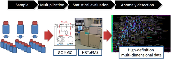
In the present study we assess the feasibility of non-target environmental monitoring that incorporates key technologies, such as simultaneous, non-target, wide-targeted, high-throughput anomaly detection and substance identification using GC×GC/ToFMS for the comprehensive, statistical analysis of river water samples.

We employed stir-bar sorptive extraction (SBSE) and total sample introduction by thermal desorption to enable comprehensive analysis with no sample loss. By omitting the pretreatment process, we effected rapid and high-throughput analysis. This approach enables the screening of substances for which no standard is available, making it possible in future automated processes to detect abnormalities by direct comparison of data. Through statistical analysis of multiple measurements of river water by GC×GC/ToFMS, we evaluated the errors inherent in the method as well as those due to sample variation.

MATERIALS AND METHODS

STANDARD REAGENTS

¹³C-labeled PAHs (16 mixtures, ES-4087, Cambridge Isotope Laboratories Inc., USA), pesticides (32 mixtures, PL1-1, Fuji Film Wako Pure Chemical Corp., Tokyo), and POPs (27 mixtures, ES-5467, CIL) as shown in Table S1.

RIVER WATER SAMPLES

Water samples were collected from monitoring sites in a small river in the Kanto region of Japan. We evaluated the reproducibility of our analysis method and the degree to which intergroup differences were detectable. The river from which the samples were taken flows through rural areas, mainly paddy fields, and is also used as an agricultural water supply. There are small facilities and residential areas near the river, but they do not appear to significantly influence the water quality. Six samples were collected in glass containers at intervals of several days in August 2015 and then transported to the laboratory at below 15°C, sealed and light-shielded. Once in the laboratory, the samples were stored at 4°C until measurement.

SAMPLE EXTRACTION

Five divided sub-samples (50 ml each) were prepared from six water samples, and a total of 30 samples were subjected to SBSE as described in several reports; for example, Ochiai et al., 2011. Acetone (PCB analysis grade, Fuji Film, Wako) and NaCl (PCB analysis grade, Kanto Chemical Co., Ltd., Tokyo) were added to the water samples in headspace vials at 10% (v/v) and 20% (w/w), respectively. A Twister^®, 20 mm long and 0.5 mm thick, coated with polydimethyl siloxane (PDMS) (Gerstel GmbH & Co. KG, Germany) was then placed in the vials, which were then sealed. The organic compounds in the samples were extracted by stirring the Twister^® with a magnetic stirrer for 24 hours. For the realization of non-target environmental monitoring, it is necessary to prevent the loss, alteration, or addition of materials during the processing of the samples; therefore, no processing—such as purification after extraction—was applied in this method (Hashimoto et al., 2011, 2018).

MEASUREMENT

Just prior to measurement, 500 pg ¹³C-PAH was added to a Twister^® and its level measured by thermal desorption (TD)-GC×GC/ToFMS. Thermal desorption was carried out using a TDU2 (Gerstel). An Agilent 7890GC (Agilent Technologies, Inc., California, USA) installed with a Zoex2006 GC×GC modulator (Zoex Corp., Texas, USA) and an Agilent 7200B QTOF were used for the measurements. The measurement conditions consisted of the EI method with a mass resolution of 10,000 (full width half maximum), a data collection period of 33 Hz, ionization voltage of 70 eV, and ionization current of 35 µA. An InertCap 5MS/Sil (45 m long, 0.25 mm I.D., 0.1 µm film thickness, GL Science Inc., Japan) was used as the first dimensional column, and a BPX-50 (0.9 m long, 0.1 mm I.D., 0.1 µm film thickness, Trajan Scientific Australia Pty Ltd, Australia) was used as the second dimensional column. These conditions are shown in Table S2.

DATA PREPARATION

The data measured by GC×GC/ToFMS were centroided (the mass spectra data were converted into bar data) using the center-of-gravity method and converted to netCDF format. The netCDF data were read using GCImage R.2.6 or R.2.7 (GC Image, LLC, Nebraska, USA) and automatic peak detection was performed based on two-dimensional total ion chromatograms (2D-TIC). Retention times of peaks on GC1 and GC2, mass spectra of the peak tops, and peak intensity in the TIC as sum of the mass spectra were used for subsequent analysis. For the purposes of this study, which is to investigate the feasibility of detecting differences from non-target analysis data, it would be redundant to conduct an analysis of all of the thousands of components (peaks) that were detected. Furthermore, it would have been impossible to analyze all components due to our use of visual confirmation of the data (manual processing). Therefore, only a proportion of the components was analyzed. Eighty is probably an adequate number, although this may be arguable. The 80 components were carefully selected based on random sampling, with the selection of those with 1) low to high boiling points, as measured in relation to retention time [RT] of GC1, 2) low to high polarity, as measured in relation to the RT of GC2, and 3) low to high concentration, as measured in relation to peak signal intensity. The RTs (primary and secondary RTs), mass spectra, and the sum of the signal intensities of the mass spectra were compared with those of the 80 components appearing at the same RT for a total of 30 data items (6 days×5). The peak alignment was performed by eye; no software processing alignment was performed. No deconvolution was carried out.

COMPARISON OF NON-TARGET MONITORING DATA FOR DETECTION OF DIFFERENCES

In this study, we attempted to detect differences (which we term here as anomaly detection) by direct comparison of non-target measurement data, rather than using the conventional method of identifying a substance and then comparing its quantitative values. This method has potential for future automated processing.

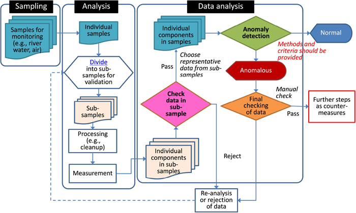
An overall workflow for anomaly detection using non-target data is shown in Fig. 1. In this study, data from GC×GC/ToFMS measurements of river water samples were used, but this workflow can be much more generally applied, irrespective of sample type or measurement method.

Fig. 1

Workflow of quality inspection of data and anomaly detection for non-target environmental monitoring

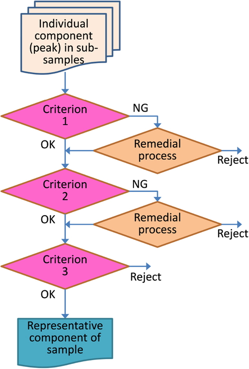
Evaluation of reproducibility was based on following three criteria, with only those components that met all the criteria being used for comparison between samples; i.e., the detection of differences between groups, anomaly detection. The evaluation flow for reproducibility is shown in Fig. 2. These criteria have been provisionally defined based on our experience of validating these methods and should be optimized for location and purpose.

Criterion 1, for checking reproducibility of GC×GC. RTs for GC1 (min) and GC2 (sec) are within ±0.25% and ±2.5%, respectively.

Criterion 2, for checking reproducibility of MS (ToFMS). The first candidate name by NIST library search is the same (instead of checking for similarity of mass spectra).

Criterion 3, to confirm the reproducibility of the entire procedure, from sample extraction (SBSE) to measurement by GC×GC/ToFMS. The relative standard deviation (RSD) of the total ion intensity (sum of mass spectral intensities of each component) is less than or equal to 15%, or the departure from the average intensity is within ±25%.

Remedial process. If outliers were below 1/5 of sub-samples, only the outliers are rejected. Otherwise, the component (peak) data are rejected.

Fig. 2

Check data in sub-samples

Criterion 1: Retention times should vary ±0.25 on GC1 and ±2.5% on GC2.

Criterion 2: Mass spectra should be the same. (The compound name obtained from the NIST library search should be the same.)

Criterion 3: Relative standard deviation (RSD) of intensities of total ions should be below 15% or the intensities should range within ±25%.

Remedial process: If outliers were below 1/5 of sub-samples, only the outliers are rejected. Otherwise, the component (peak) data is rejected.

Calculations and comparisons for criteria 1 and 3 were carried out on an Excel spreadsheet (Microsoft Corp., USA). For comparison of the mass spectra of criterion 2, we emphasized simplicity rather than statistical methods, and used the substance names (or CAS. Nos.) that were listed as first candidates as a result of a normal search of the NIST14 (National Institute of Standards and Technology, USA) mass library using MS Search 2.0 (NIST). In other words, the results were judged according to whether or not the compound name hit as the first candidate were identical.

For the components that passed all of the above reproducibility evaluation criteria, we examined whether differences between samples could be detected. The Kruskal-Wallis test, a nonparametric between-group difference test method, was used to evaluate the inter-sample differences. The calculations were performed on EZR 1.35 statistical software (Kanda, 2013) using R Commander version 2.2.3.

RESULTS AND DISCUSSION

INVESTIGATION OF EXTRACTION CONDITIONS FOR SOLID PHASE OF AGITATOR

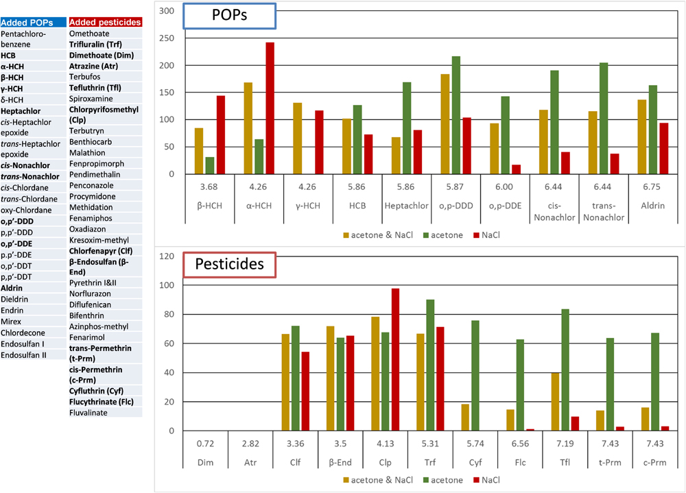
SBSE conditions were investigated to enable detection of compounds with a wide range of physicochemical properties. A 5-μl acetone solution containing 28 POPs and 32 pesticides at 200–400 pg each was added to 50 ml of river water to check the recovery rate of SBSE. Log K_ow of the standards used ranged from 0.72–7.43, which can be considered a relatively wide range. The recovery rate was calculated by subtracting the quantities of compounds originally present in the river water (the control values) due to the addition of non-labeled pesticides to the river water in the recovery study.

In Fig. 3 we show the effect of the additive on the recovery of POPs and pesticides. The green, red, and yellow bars in the graphs show recovery rates when 20% (v/v) acetone, 10% (w/w) NaCl, or both, were added to water before extraction. Our results indicate that the recovery of high-log K_ow compounds is notably high when acetone is added, whereas the recovery of low-log K_ow compounds is high with the addition of NaCl. We confirmed that a relatively wide range of compounds with log K_ow could be extracted by adding both acetone and NaCl. Although it is somewhat difficult to interpret the recovery rate of pesticides, it is assumed that those from river samples were influenced by the complex matrix of river water. Although it was difficult to achieve high recoveries of all the compounds, the addition of both acetone and NaCl was adopted for the purpose of detecting a wide range of compounds. Another reason for the considerable variability in recovery rates may be the low reproducibility of SBSE. In this study, we used general conditions that can capture a wide range of chemical properties from low (approximately 2) to high (approximately 12) log K_ow, but there may have been a lack of stability. In the future, it will be necessary to improve the reproducibility of the system. Here we estimated the variability simultaneously by setting n=5 for the extracted samples.

Fig. 3

Recoveries (%) of POPs and pesticides by SBSE from a river water sample

SBSE: Stir-bar solid-phase extraction, acetone: 20% (v/v), NaCl: 10% (w/w)

As example, recoveries of 11 of 28 POPs and 11 of 32 pesticides were shown.

Value in upper of substance name indicates log Kow.

DETECTION OF DIFFERENCES IN NON-TARGET MONITORING DATA (PRECISION MASS SPECTRA)

For environmental non-target monitoring, a time-series comparison of GC×GC/ToFMS measurement data was performed. With the conventional method, many (or most) components cannot be identified, and identification of a single substance is a time-consuming process. However, the new method has the advantages of rapidity without data omissions or misidentification and has the potential for automation in the future.

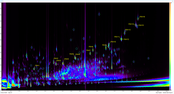
As an example, as shown in Fig. 4, more than 2,000 components were detected in all the samples. In actual environmental monitoring, it would be necessary to detect anomalies in all of them. To validate our method, we focused on those that covered the entire area on the 2D chromatogram and had an intensity that ranged from around the detection limit to the maximum level. Qualitative and quantitative reproducibility and inter-sample differences were evaluated for 80 selected components. The components (peaks) were selected based on 2D-TIC, and the mass spectra of the peak tops were analyzed and examined. The ultimate goal is to detect anomalies by direct comparison of the measured data (Fig. S1). It is theoretically possible to compare the mass spectra of all data points using the same procedure. However, in this case, very strict alignment of retention times would be required. The next best solution is to divide the retention time plane into a grid and compare the mass spectrum in each grid. We hope to address this question in the next stage of our research.

Fig. 4

An example of a two-dimensional total ion chromatogram of river water sample measured by TD/GCxGC/ToFMS

Eighty peaks marked with green circles (〇) were evaluated quantitatively and qualitatively for reproducibility.

Sixteen ¹³C-labeled PAHs are shown by PAH+number

The measurement reproducibility of the divided sample (n=5) was first evaluated for 80 of the detected components. The higher the reproducibility, the more reliable the method and the more sensitive and accurate was the anomaly detection. We confirmed reproducibility for components that met all three previously presented criteria before making comparisons among samples (intergroup differences, anomaly detection).

For the results of the comprehensive analysis of water quality over six days, the pass rate of each criterion was calculated as the ratio of 80 components×5 divisions to the total number of 400. The pass rates of criteria 1, 2, and 3 were 51%–75%, 39%–53%, and 22%–43%, respectively (Fig. S2). At this time, when the remedial data number, excluding outliers, was four or more and criteria 2 and 3 were satisfied, the pass rates for criteria 1 and 2 improved to 66%–89% and 56%–78%, respectively, as shown in “passed + revival” in Fig. S2. Here criterion 1 indicates the reproducibility of GC×GC, criterion 2 indicates the reproducibility of ToFMS, and criterion 3 indicates the reproducibility of the whole procedure, from sample extraction by SBSE to measurement by GC×GC/ToFMS. The low pass rate of criterion 3 indicates that the reproducibility of the entire method is problematic, making it necessary to correct our extraction and heating/desorption methods and improve the sensitivity. In this case, the addition of an internal standard before the extraction operation and the sensitivity correction by the measured value can be regarded as one method, but the question of what internal standard and how to select it is a problem for non-target analysis.

In Table S3 we present a list of RSDs for TIC intensity (n=5) for 80 components. We note that when the threshold was set to 50% or less RSD, approximately 60% of 480 (323) could be passed. The components with high RSD (poor reproducibility) were biased. For example, there was extremely poor reliability in detecting component IDs: chk09, 10, 13, 34, and 67, with large RSDs in all the 6-day samples. The measured values of individual components appear to be highly variable, so attention should be paid to the risk of erroneous environmental assessment and environmental monitoring if SBSE is employed without taking the reproducibility of the method into consideration.

Because the handling of mass errors is also a concern when dealing with accurate mass data, we substituted the NIST library search results to mitigate the effect of mass errors; i.e., integer masses were rounded and the calculation of the mass spectral similarity was simplified. We are currently developing and testing a method of calculating the mass error and the similarity of mass spectra. We will report on this method in the near future.

EVALUATION OF THE DETECTABILITY OF DIFFERENCES

We assessed the detectability of inter-sample differences for the components that passed up to criterion 2 (56–78% pass rate, including the remedy). The Kruskal-Wallis test, a nonparametric intergroup difference test method, was used to evaluate the inter-sample differences. The original plan was to test for inter-sample differences in the data that passed up to criterion 3, but as mentioned above, the rate of passing up to criterion 3 was low, so we extended the scope to the data that passed up to criterion 2. Another reason for this was to confirm the sensitivity and robustness of detection of inter-sample differences.

In Table S4 we list the results of the Kruskal-Wallis test for the p-values of the 80 components that met criterion 2. A smaller p-value indicates a significant inter-sample difference. As a result, there were 40 components with a p-value of less than 0.01, which is more than half of the components tested, and 53/75, approximately 70% of the components, with a p-value of less than 0.05. This indicates that differences between samples can be detected for many components, even if the variability of the measured values is relatively large (RSD>15%).

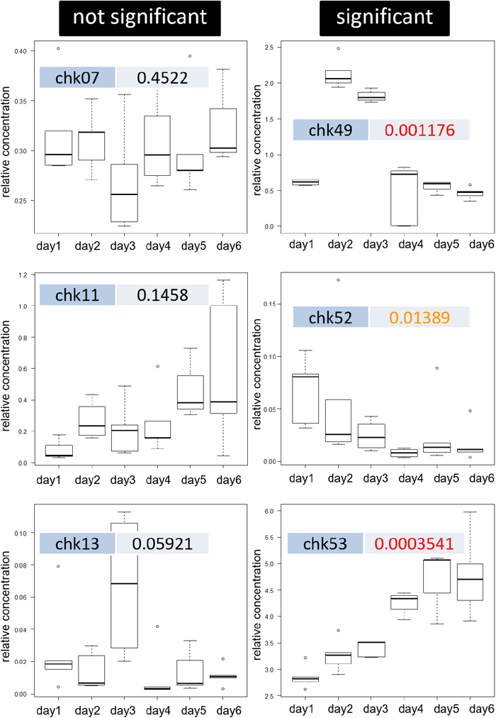
In Fig. 5 we give an example of a quartile graph of the total ion signal intensity for each component. Significant differences can be seen in chk49, 52, and 53, shown in the Figure (right). Some of the components that showed significant differences in the test showed an increasing or decreasing trend over time. As shown in Table S5, a library search of NIST14 revealed the match factor of these components to be 700 or higher, with a rising trend seen for the typical examples of butylhydroxytoluene (CAS No. 128-37-0), 2,2,2,4-trimethyl-1,3-pentanediol diisobutyrate (CAS No. 6846-50-0), and methyl 2-benzoylbenzoate (CAS No. 606-28-0). Those with a decreasing trend were 2,3,4,5,6-pentachloroaniline (CAS No. 527-20-8), p-isopropenylphenol (CAS No. 4286-23-1), and benzo[k]fluoranthene (CAS No. 207-08-9).

Fig. 5

Examples of variation of intensities in sub-samples as box-charts

Significant; p<0.05 obtained by Kruskal-Wallis test

We confirmed that differences among samples can be detected even if the variation in measured values is relatively large, which suggests considerable potential for the development of a relatively robust anomaly detection method. We expect that it would be possible in the future to implement non-target environmental monitoring by removing and stabilizing the variables from sampling to measurement, simplifying multivariate comparisons and reducing resources, and automating the entire process.

The purpose of this study was to determine whether SBSE-TD-GC×GC/ToFMS non-target analysis can be applied to environmental monitoring and to identify problems with the application of this method. General conditions are adopted that are least likely to be missed and which will capture a wide range of chemicals. We also believe that, in practice, it is necessary to narrow down the target constituents based on the characteristics of each monitoring point. Aside from the question of whether the exclusion of matrices matches the purpose of non-target analysis, it may be possible to reduce the number of matrices by increasing the selectivity of SBSE while changing the adsorbent and/or adding solvent, or by adding solvent extraction and certain pre-treatments. Post-data processing, which we have developed (Zushi et al., 2017, 2018), is also a potential solution.

CONCLUSION

In this study, we have described a rapid and comprehensive environmental monitoring method that uses GC/MS and have proposed methods for its practical application. The rapid and comprehensive GC×GC/ToFMS method developed in the previous study, which greatly reduces the need for pretreatment, was applied to actual continuous measurement of river water. The water samples were analyzed by sorptive extraction using a magnetic stirrer coated with polydimethyl siloxane, and direct and whole sample extracts were determined by thermal desorption/comprehensive (GC×GC)/ToFMS (TD/GC×GC/ToFMS). It was confirmed by statistical methods, such as nonparametric multigroup comparisons, that differences can be detected even when comparing raw data without substance identification. In other words, it was shown that a change in concentration (signal intensity) of an unknown substance can be detected.

We observed a number of limitations that should be addressed in the application of the method. Variations in data (retention time, mass, and intensity) affect the ability to detect differences, so the accuracy of each of these needs to be improved to be able to detect small differences. Improving the reproducibility of extraction rates and selecting internal standards for concentration corrections are major challenges in non-target environmental monitoring. The results of this study using multiple measurements also reaffirmed the danger of environmental assessment and environmental monitoring based on n=1 analysis value without taking method reproducibility into account.

With this study we have described a first step in exploring whether difference detection based on instrumental measurement data is possible for non-target environmental monitoring. The results presented here are therefore only a general framework for the process. Further examinations and empirical testing of the methods and conditions are needed to transform the general method into standard operating procedures.

ACKNOWLEDGMENTS

We thank the staff of Center for Environmental Science in Saitama for river sample collection. This work was supported by JSPS Kakenhi Grant Number 17H00796.

SUPPLEMENTARY MATERIAL

Table S1, List of standard compounds used in this study; Table S2, Instrumental conditions used in this study; Table S3, Relative standard deviations (%) of intensity of sub-samples of 80 components evaluated for method reproducibility; Table S4, Detection of differences among samples as results of Kruskal-Wallis test; Table S5, Results of NIST14 library searching of 80 components in river water; Fig. S1, Conceptual diagram of comparison of data and time; Fig. S2, Result of check data in sub-samples.

This material is available on the Website at https://doi.org/10.5985/emcr.20200001.

REFERENCES

•  Alexandrino,  G.L.,  Tomasi,  G.,  Kienhuis,  P.G.M.,  Augusto,  F.,  Christensen,  J.H., 2019. Forensic investigations of diesel oil spills in the environment using comprehensive two-dimensional gas chromatography–high resolution mass spectrometry and chemometrics: new perspectives in the absence of recalcitrant biomarkers. Environ. Sci. Technol. 53, 550–559. doi: 10.1021/acs.est.8b05238.
•  Bletsou,  A.A.,  Jeon,  J.,  Hollender,  J.,  Archontaki,  E.,  Thomaidis,  N.S., 2015. Targeted and non-targeted liquid chromatography-mass spectrometric workflows for identification of transformation products of emerging pollutants in the aquatic environment. TrAC Trends Anal. Chem. 66, 32–44. doi: 10.1016/j.trac.2014.11.009.
•  Brack,  W.,  Ait-Aissa,  S.,  Burgess,  R.M.,  Busch,  W.,  Creusot,  N.,  Di Paolo,  C.,  Escher,  B.I.,  Mark Hewitt,  L.,  Hilscherova,  K.,  Hollender,  J.,  Hollert,  H.,  Jonker,  W.,  Kool,  J.,  Lamoree,  M.,  Muschket,  M.,  Neumann,  S.,  Rostkowski,  P.,  Ruttkies,  C.,  Schollee,  J.,  Schymanski,  E.L.,  Schulze,  T.,  Seiler,  T.B.,  Tindall,  A.J.,  De Aragão Umbuzeiro,  G.,  Vrana,  B.,  Krauss,  M., 2016. Effect-directed analysis supporting monitoring of aquatic environments—an in-depth overview. Sci. Total Environ. 544, 1073–1118. doi: 10.1016/j.scitotenv.2015.11.102.
•  Brack,  W.,  Altenburger,  R.,  Schüürmann,  G.,  Krauss,  M.,  López Herráez,  D.,  van Gils,  J.,  Slobodnik,  J.,  Munthe,  J.,  Gawlik,  B.M.,  van Wezel,  A.,  Schriks,  M.,  Hollender,  J.,  Tollefsen,  K.E.,  Mekenyan,  O.,  Dimitrov,  S.,  Bunke,  D.,  Cousins,  I.,  Posthuma,  L.,  van den Brink,  P.J.,  López de Alda,  M.,  Barceló,  D.,  Faust,  M.,  Kortenkamp,  A.,  Scrimshaw,  M.,  Ignatova,  S.,  Engelen,  G.,  Massmann,  G.,  Lemkine,  G.,  Teodorovic,  I.,  Walz,  K.H.,  Dulio,  V.,  Jonker,  M.T.,  Jäger,  F.,  Chipman,  K.,  Falciani,  F.,  Liska,  I.,  Rooke,  D.,  Zhang,  X.,  Hollert,  H.,  Vrana,  B.,  Hilscherova,  K.,  Kramer,  K.,  Neumann,  S.,  Hammerbacher,  R.,  Backhaus,  T.,  Mack,  J.,  Segner,  H.,  Escher,  B.,  de Aragão Umbuzeiro,  G., 2015. The SOLUTIONS project: challenges and responses for present and future emerging pollutants in land and water resources management. Sci. Total Environ. 503–504, 22–31. doi: 10.1016/j.scitotenv.2014.05.143.
•  Cervera,  M.I.,  Portolés,  T.,  Pitarch,  E.,  Beltrán,  J.,  Hernández,  F., 2012. Application of gas chromatography time-of-flight mass spectrometry for target and non-target analysis of pesticide residues in fruits and vegetables. J. Chromatogr. A 1244, 168–177. doi: 10.1016/j.chroma.2012.04.063.
•  Eljarrat,  E.,  Barcelo,  D., 2006. Quantitative analysis of polychlorinated n-alkanes in environmental samples. TrAC Trends Anal. Chem. 25, 421–434. doi: 10.1016/j.trac.2006.01.007.
•  Focant,  J.F.,  Sjödin,  A.,  Patterson,  D.G., 2003. Qualitative evaluation of thermal desorption-programmable temperature vaporization-comprehensive two-dimensional gas chromatography–time-of-flight mass spectrometry for the analysis of selected halogenated contaminants. J. Chromatogr. A 1019, 143–156. doi: 10.1016/j.chroma.2003.07.007.
•  Fushimi,  A.,  Hashimoto,  S.,  Ieda,  T.,  Ochiai,  N.,  Takazawa,  Y.,  Fujitani,  Y.,  Tanabe,  K., 2012. Thermal desorption - comprehensive two-dimensional gas chromatography coupled with tandem mass spectrometry for determination of trace polycyclic aromatic hydrocarbons and their derivatives. J. Chromatogr. A 1252, 164–170. doi: 10.1016/j.chroma.2012.06.068.
•  García-Reyes,  J.F.,  Hernando,  M.D.,  Molina-Díaz,  A.,  Fernández-Alba,  A.R., 2007. Comprehensive screening of target, non-target and unknown pesticides in food by LC-TOF-MS. TrAC-Trends Anal. Chem. 26, 828–841. doi: 10.1016/j.trac.2007.06.006.
•  Hashimoto,  S.,  Honda,  M.,  Takasuga,  T.,  Ubukata,  M.,  Tanaka,  K.,  Tanabe,  K.,  Shibata,  Y., 2010. Measurement of hydroxy PCB by a comprehensive multi dimensional gas chromatogragh-time-of-flight mass spectrometer. J. Environ. Chem. 20, 161–172. doi: 10.5985/jec.20.161.
•  Hashimoto,  S.,  Takazawa,  Y.,  Fushimi,  A.,  Ito,  H.,  Tanabe,  K.,  Shibata,  Y.,  Ubukata,  M.,  Kusai,  A.,  Tanaka,  K.,  Otsuka,  H.,  Anezaki,  K., 2008. Quantification of polychlorinated dibenzo-p-dioxins and dibenzofurans by direct injection of sample extract into the comprehensive multidimensional gas chromatograph/high-resolution time-of-flight mass spectrometer. J. Chromatogr. A 1178, 187–198. doi: 10.1016/j.chroma.2007.11.067.
•  Hashimoto,  S.,  Takazawa,  Y.,  Fushimi,  A.,  Tanabe,  K.,  Shibata,  Y.,  Ieda,  T.,  Ochiai,  N.,  Kanda,  H.,  Ohura,  T.,  Tao,  Q.,  Reichenbach,  S.E., 2011. Global and selective detection of organohalogens in environmental samples by comprehensive two-dimensional gas chromatography-tandem mass spectrometry and high-resolution time-of-flight mass spectrometry. J. Chromatogr. A 1218, 3799–3810. doi: 10.1016/j.chroma.2011.04.042.
•  Hashimoto,  S.,  Zushi,  Y.,  Fushimi,  A.,  Takazawa,  Y.,  Tanabe,  K.,  Shibata,  Y., 2013. Selective extraction of halogenated compounds from data measured by comprehensive multidimensional gas chromatography/high resolution time-of-flight mass spectrometry for non-target analysis of environmental and biological samples. J. Chromatogr. A 1282, 183–189. doi: 10.1016/j.chroma.2013.01.052.
•  Hashimoto,  S.,  Zushi,  Y.,  Takazawa,  Y.,  Ieda,  T.,  Fushimi,  A.,  Tanabe,  K.,  Shibata,  Y., 2018. Selective and comprehensive analysis of organohalogen compounds by GC×GC–HRTofMS and MS/MS. Environ. Sci. Pollut. Res. 25, 7135–7146. doi: 10.1007/s11356-015-5059-5.
•  Ibáñez,  M.,  Sancho,  J.V.,  Hernández,  F.,  McMillan,  D.,  Rao,  R., 2008. Rapid non-target screening of organic pollutants in water by ultraperformance liquid chromatography coupled to time-of-light mass spectrometry. TrAC-Trends Anal. Chem. 27, 481–489. doi: 10.1016/j.trac.2008.03.007.
•  Ieda,  T.,  Hashimoto,  S.,  Isobe,  T.,  Kunisue,  T.,  Tanabe,  S., 2019. Evaluation of a data-processing method for target and non-target screening using comprehensive two-dimensional gas chromatography coupled with high-resolution time-of-flight mass spectrometry for environmental samples. Talanta 194, 461–468. doi: 10.1016/j.talanta.2018.10.050.
•  Kanda,  Y., 2013. Investigation of the freely available easy-to-use software ‘EZR’ for medical statistics. Bone Marrow Transplant. 48, 452–458. doi: 10.1038/bmt.2012.244.
•  Lješević,  M.,  Gojgić-Cvijović,  G.,  Ieda,  T.,  Hashimoto,  S.,  Nakano,  T.,  Bulatović,  S.,  Ilić,  M.,  Beškoski,  V., 2019. Biodegradation of the aromatic fraction from petroleum diesel fuel by Oerskovia sp. followed by comprehensive GC×GC-TOF MS. J. Hazard. Mater. 363, 227–232. doi: 10.1016/j.jhazmat.2018.10.005.
•  Muscalu,  A.M.,  Morse,  D.,  Reiner,  E.J.,  Górecki,  T., 2017. The quantification of short-chain chlorinated paraffins in sediment samples using comprehensive two-dimensional gas chromatography with μECD detection. Anal. Bioanal. Chem. 409, 2065–2074. doi: 10.1007/s00216-016-0153-1.
•  Ochiai,  N.,  Ieda,  T.,  Sasamoto,  K.,  Takazawa,  Y.,  Hashimoto,  S.,  Fushimi,  A.,  Tanabe,  K., 2011. Stir bar sorptive extraction and comprehensive two-dimensional gas chromatography coupled to high-resolution time-of-flight mass spectrometry for ultra-trace analysis of organochlorine pesticides in river water. J. Chromatogr. A 1218, 6851–6860. doi: 10.1016/j.chroma.2011.08.027.
•  Rezek,  J.,  Macek,  T.,  Doubsky,  J.,  Mackova,  M., 2012. Metabolites of 2,2′-dichlorobiphenyl and 2,6-dichlorobiphenyl in hairy root culture of black nightshade Solanum nigrum SNC-9O. Chemosphere 89, 383–388. doi: 10.1016/j.chemosphere.2012.05.041.
•  Schymanski,  E.L.,  Singer,  H.P.,  Slobodnik,  J.,  Ipolyi,  I.M.,  Oswald,  P.,  Krauss,  M.,  Schulze,  T.,  Haglund,  P.,  Letzel,  T.,  Grosse,  S.,  Thomaidis,  N.S.,  Bletsou,  A.,  Zwiener,  C.,  Ibáñez,  M.,  Portolés,  T.,  de Boer,  R.,  Reid,  M.J.,  Onghena,  M.,  Kunkel,  U.,  Schulz,  W.,  Guillon,  A.,  Noyon,  N.,  Leroy,  G.,  Bados,  P.,  Bogialli,  S.,  Stipaničcev,  D.,  Rostkowski,  P.,  Hollender,  J., 2015. Non-target screening with high-resolution mass spectrometry: critical review using a collaborative trial on water analysis. Anal. Bioanal. Chem. 407, 6237–6255. doi: 10.1007/s00216-015-8681-7.
• Solutions Project, 2004. Solutions Project Web page [WWW Document]. https://www.solutions-project.eu/ (accessed 1 February 2021)
• The NORMAN Network, 2012. The NORMAN network Web page [WWW Document]. https://www.norman-network.net/ (accessed 1 February 2021)
•  Tian,  Z.,  Peter,  K.T.,  Gipe,  A.D.,  Zhao,  H.,  Hou,  F.,  Wark,  D.A.,  Khangaonkar,  T.,  Kolodziej,  E.P.,  James,  C.A., 2020. Suspect and nontarget screening for contaminants of emerging concern in an urban estuary. Environ. Sci. Technol. 54, 889–901. doi: 10.1021/acs.est.9b06126.
•  Tran,  C.D.,  Dodder,  N.G.,  Quintana,  P.J.E.,  Watanabe,  K.,  Kim,  J.H.,  Hovell,  M.F.,  Chambers,  C.D.,  Hoh,  E., 2020. Organic contaminants in human breast milk identified by non-targeted analysis. Chemosphere 238, 124677. doi: 10.1016/j.chemosphere.2019.124677.
• United States Environmental Protection Agency [USEPA], 1991. Technical support document for water quality-based toxic control. Epa-505/ 2, 90/001.
•  Yamamoto,  H.,  Niino,  T.,  Tatarazako,  N., 2015. Current trends and future perspectives on evaluation and control of toxic chemicals in effluents using bioassay. J. Environ. Chem. 25, 3–10. doi: 10.5985/jec.25.3.
•  Zushi,  Y.,  Gros,  J.,  Tao,  Q.,  Reichenbach,  S.E.,  Hashimoto,  S.,  Arey,  J.S., 2017. Pixel-by-pixel correction of retention time shifts in chromatograms from comprehensive two-dimensional gas chromatography coupled to high resolution time-of-flight mass spectrometry. J. Chromatogr. A 1508, 121–129. doi: 10.1016/j.chroma.2017.05.065.
•  Zushi,  Y.,  Hashimoto,  S., 2018. Direct classification of GC×GC-analyzed complex mixtures using non-negative matrix factorization-based feature extraction. Anal. Chem. 90, 3819–3825. doi: 10.1021/acs.analchem.7b04313.
•  Zushi,  Y.,  Hashimoto,  S.,  Fushimi,  A.,  Takazawa,  Y.,  Tanabe,  K.,  Shibata,  Y., 2013. Rapid automatic identification and quantification of compounds in complex matrices using comprehensive two-dimensional gas chromatography coupled to high resolution time-of-flight mass spectrometry with a peak sentinel tool. Anal. Chim. Acta 778, 54–62. doi: 10.1016/j.aca.2013.03.049.
•  Zushi,  Y.,  Hashimoto,  S.,  Tamada,  M.,  Masunaga,  S.,  Kanai,  Y.,  Tanabe,  K., 2014. Retrospective analysis by data processing tools for comprehensive two-dimensional gas chromatography coupled to high resolution time-of-flight mass spectrometry: A challenge for matrix-rich sediment core sample from Tokyo Bay. J. Chromatogr. A 1338, 117–126. doi: 10.1016/j.chroma.2014.02.015.
•  Zushi,  Y.,  Hashimoto,  S.,  Tanabe,  K., 2015. Global spectral deconvolution based on non-negative matrix factorization in GC×GC-HRTOFMS. Anal. Chem. 87, 1829–1838. doi: 10.1021/ac5038544.