Abstract
The sulfur isotope fractionation that occurs during SO2 photolysis is key to explaining the isotope signatures stored in ancient sedimentary rocks and understanding the atmospheric compositions of the early Earth and early Mars. Here, we report the photoabsorption cross-sections of 32SO2, 33SO2, 34SO2, and 36SO2 measured from 206 to 220 nm at 296 K. The wavelength resolution was set to 1 cm–1, 25 times higher than that of previous SO2 isotopologue absorption spectra measurements. The precision of ~10% is in agreement with previously reported SO2 absorption spectra. In comparison with previously reported high-resolution spectra of natural abundance, SO2 measurements demonstrate smaller cross-sectional magnitudes at absorption peaks and an offset wavelength by ~0.016 nm. Using the newly recorded isotopologue spectra, we calculated the sulfur isotope fractionation for self-shielding during SO2 photolysis. The calculated 34S fractionation (34ε) roughly reproduces the observed relationship between 34ε and the SO2 column density in previous photolysis experiments. Thus, the cross-section is useful for predicting 34S/32S isotope fractionation in an optically thick SO2 atmosphere. In contrast, for mass-independent fractionation (MIF-S, i.e., non-zero Δ33S), the measured spectra predicted a weakly negative Δ33S/δ34S slope of about –0.1. The small Δ33S/δ34S slope is consistent with the slopes of SO2 photolysis experiments under high-pressure atmospheres (i.e., the pressure broadened absorption line width will be comparable to the spectral resolution). Therefore, MIF-S during photolysis experiments was linked to spectroscopic measurements for the first time. We conclude that reasonable precision and high-resolution spectroscopic measurements are key to explaining the origin of MIF-S at column densities below 1018 cm–2. However, MIF-S production in chamber experiments or atmospheric conditions may require understanding pressure or temperature effects, such as linewidth broadening on the UV-absorption spectra, and how these effects manifest themselves on isotopologues.
Introduction
Sulfur dioxide (SO2) plays an important role in planetary atmospheres, including that of the Earth. This gas has been released into the atmosphere by volcanic activity throughout Earth’s history (Holland, 2002; Gaillard et al., 2011; Olson et al., 2019; Ohmoto, 2020), is a candidate greenhouse gas in early Mars (Halevy et al., 2007; Johnson et al., 2008), and has also been observed in Venus and Io’s atmospheres (e.g., Vandaele et al., 2017; Feaga et al., 2009).
SO2 has two strong structured absorption bands in the UV region; therefore, UV radiation triggers complex photochemical processes in this molecule (e.g., Heicklen et al., 1980). The 165–230 nm absorption band occurs where SO2 is photolyzed by wavelengths below 218.7 nm (Katagiri et al., 1997) by its excitation to the C1B2 state. The second absorption band occurs in the 250–340 nm region, where SO2 is excited to the B(1B1 + 1A2) state. In the oxygen-free and ozone-free atmosphere of the early Earth, photons above approximately 190 nm penetrated the troposphere (Ueno et al., 2009), making complex light-induced chemistry possible for this molecule.
SO2 photolysis originates large mass-independent fractionation of sulfur isotopes (MIF-S), which is notably distinct from the more commonly observed mass-dependent fractionation (e.g., Farquhar et al., 2001; Whitehill and Ono, 2012; Franz et al., 2013; Ono, 2017). Specifically, MIF-S has been found in Archean sedimentary rocks (e.g., Farquhar et al., 2000a), Martian meteorites (e.g., Farquhar et al., 2000b), sulfate aerosols in polar ice (e.g., Savarino et al., 2003), and in the present atmosphere (e.g., Romero and Thiemens, 2003). The Archean MIF-S may provide insights into the atmospheric chemical composition at that time (e.g., Ono, 2017). Previous laboratory experiments and numerical modeling suggest that MIF-S reflects various atmospheric parameters: very low partial pressure (<2 ppm) of O2 is required to preserve the MIF-S signatures (Δ33S≠0) in both sulfide and sulfate minerals (Pavlov and Kasting, 2002; Zahnle et al., 2006); SO2 column density (or partial pressure of SO2) changes Δ33S and Δ36S magnitudes (Ono et al., 2013); atmospheric pressure changes Δ36S/Δ33S slope (Lyons et al., 2018; Endo et al., 2019); reducing gases such as hydrocarbons and carbon monoxide (CO) changes the Δ36S/Δ33S slope by MIF-S in SO2-photoexcitation chemistry (Whitehill et al., 2013; Endo et al., 2016; Kroll et al., 2018); and strong UV absorption, such as by organic haze, changes the branching ratios of SO2 photolysis/photoexcitation and MIF-S (Zerkle et al., 2012). In addition, the polymerization of elemental sulfur, excluding SO2 photochemistry, has also been proposed as an MIF-S mechanism (Babikov, 2017; Harman et al., 2018; Lin and Thiemens, 2020).
The most common feature of the Archean geologic MIF-S is a Δ36S/Δ33S-slope of ~–0.9 (Farquhar et al., 2000a). Recently, Endo et al. (2016) and Mishima et al. (2017) argued that this can be explained by mixing MIF-S during SO2 photolysis (Δ36S/Δ33S ~ –2.4) with MIF-S induced during SO2 photoexcitation (Δ36S/Δ33S ~ +0.8). A highly reducing atmosphere, such as Earth’s ancient atmosphere containing a significant percentage of carbon monoxide or methane, is required to propagate MIF-S induced by SO2 photoexcitation. Independently, a highly reducing atmosphere is also speculated based on xenon isotopes (Avice et al., 2018; Zahnle et al., 2019). However, the second most basic trend, Δ33S/δ34S (~+0.9; Ono et al., 2009), cannot be explained. The mechanisms underlying MIF-S still require further exploration.
In the present study, we focused on MIF-S during SO2 photolysis, although SO2 photoexcitation also causes a large MIF-S (Whitehill et al., 2013). The underlying mechanisms of MIF-S in the photoexcitation are likely isotopologue-specific perturbations (Whitehill et al., 2013), and the mechanisms may also occur in isotope fractionation during N2 and CO photolysis (Chakraborty et al., 2008, 2014). The MIF-S during SO2 photolysis is dependent on the SO2 column density and total pressure. This relationship can be explained by decreasing 32SO2 (and possibly 33SO2 at high pressure, i.e., significant pressure broadening in SO2 absorption lines) photolysis rates due to SO2 own absorption. This process is known as self-shielding or isotopic self-shielding (Ono et al., 2013; Lyons et al., 2018; Endo et al., 2019). The nature of self-shielding was recently summarized and reviewed by Lyons (2020) and Thiemens and Lin (2021). Isotope fractionation in photolysis is predicted by the absorption cross-sections of isotopologues (Miller and Yung, 2000). A small MIF-S was predicted for optically thin SO2 (i.e., without self-shielding) based on high-precision and low-wavelength resolution 32SO2, 33SO2, 34SO2, and 36SO2 (hereafter 32,33,34,36SO2) absorption spectra (Endo et al., 2015; Izon et al., 2017); this was consistent with the results of SO2-photolysis experiments (Endo et al., 2016). In principle, a large MIF-S at optically thick SO2 (i.e., with self-shielding) can also be predicted; however, predictions by absorption measurements for cross-sections of SO2 isotopologues did not match the MIF-S observed using SO2-photolysis experiments (Ono et al., 2013). This discrepancy is likely caused by the complex ro-vibrational structures of SO2-absorption spectra and the insufficient wavelength resolutions of spectroscopic measurements.
In this study, we report reasonable precision and high-resolution measurements of UV-absorption spectra of 32,33,34,36SO2 isotopologues using isotope enrichment samples. The experimental device used in this report was a full-vacuum fast Fourier transform (FFT) spectrometer with a wavelength resolution of 1 cm–1. This was ~25 times higher than that in previous reports of SO2 isotopologues (Danielache et al., 2008; Endo et al., 2015), and ~8 times lower than that reported by a previous study that used the highest resolution to measure the natural abundance of SO2 (Stark et al., 1999). Due to the trade-off between resolution and precision, the precision used was ~10 times lower than that of previous studies using a dual-beam monochromator to attain high-precision measurements (Endo et al., 2015). Absorption spectra were measured from 206 to 220 nm with sufficient precision, although most of the SO2 was photolyzed by photons from 190 to 220 nm in the Archean atmosphere. Although uncertainty remains as a result of this, the fractionation factors predicted by this study are comparable with isotope compositions of products used in previous SO2-photolysis experiments at optically thick SO2 conditions in which self-shielding occurs. In addition, we compared the results with a simple analytical self-shielding model for the Archean MIF-S. This simple model allowed us to predict the large enrichment or depletion of clumped isotope signatures caused by self-shielding. In sum, we attempted to link sulfur isotope fractionations during photolysis experiments to spectroscopic measurements and discuss the Archean MIF-S trend produced by self-shielding.
Methods
Experimental samples
The samples measured in this report were previously presented and described in detail by Danielache et al. (2012). To ensure the isotopic purity of the samples, CuO and elemental 32S, 33S, 34S, and 36S sealed in a quartz tube under vacuum were heated at 950°C for 15 min. The resultant 32,33,34,36SO2 gas and unreacted O2 were separated using freeze-pump-thaw cycling and further purified using gas chromatography. The stability of the samples during long storage periods was maintained using sealed preheated Pyrex tubes, and the tubes were stored in a dark environment. During the experiments, when samples were used on a daily basis, containers consisting of stainless steel (SUS316) tubing welded to a bellows-sealed valve (SS-4H-TH3, Swagelok Company, U.S.A.) were used.
Spectrometry and measurements
The absorption cross-sections were determined using an FFT spectrometer (VERTEX80v, Bruker Inc., U.S.A.) equipped with a deuterium lamp (L6301-50, Hamamatsu Photonics K.K., Japan), a 10.0-cm long cell with UV-grade LiF windows, and a VUV-diode detector and calcium fluoride beam splitter. The inside of the spectrometer was constantly evacuated by a dry pump, and the interferometer was operated under a constant nitrogen gas flow. The wavelength scale of this study was calibrated using a He–Ne laser (15,798 cm–1) and water absorption lines (1554.353 and 7306.74 cm–1). Under these experimental conditions, a spectral resolution of 1 cm–1 yielded signal-to-noise ratios (SNRs) of ~20 and ~100 at 206 and 220 nm, respectively.
The SO2 cross-section is known to vary more than one order of magnitude within the measured wavelength range. To maximize the SNR conditions for all wavelengths, the sample gas pressures were set between 15 and 300 Pa by diffusion in a vacuum line. Pressures were measured using two capacitance manometers (CMR362, 0.01–110 Pa range and CMR364, 1–1.1 × 10⁴ Pa range; Pfeiffer Vacuum GmbH, Germany). The resolution and accuracy of both manometers were 0.003 and 0.2% at full scale and reading, respectively. Inaccuracies in pressure measurements induce an uncertainty of approximately ≤0.5% of the estimated cross-section. The measurements took approximately 15 min, and during this process, the sample gas pressure gradually decreased (maximum 0.3 Pa), potentially due to adsorption to the gas cell and the stainless steel vacuum line. The sample pressure utilized was the average of the pressures before and after the measurement. We assigned a conservative maximum uncertainty of 1% from the pressure.
The absorption spectrum was obtained from photon intensity spectra of the empty cell and sample. The photon intensity spectra were calculated from 100 interferograms at a resolution of 1 cm–1. A Blackman–Harris three-term apodization function, a Fourier transform window from 0 to 60,000 cm–1, and a zero-filling factor of 2 were used to produce a spectrum with an energy range of 54,000 to 35,000 cm–1 with a data point spacing of 0.241085 cm–1. Background intensity spectra (Ivacuum) and gas sample spectra (Isample) were measured in an alternating fashion.
The amplitude drift of the signal can be assessed by comparing the two background spectra. The average signal drift between 206 and 220 nm was calculated to be ~15%. A moving average of 41 points was introduced to reduce noise in the background spectra. In contrast, no such smoothing procedure was implemented for the sample spectra (Isample).
In our previous reports (Danielache et al., 2008, 2012), the background spectra at the time of the measurement were taken as the average spectra of the empty cell before (Ivacuum-before) and after (Ivacuum-after) recording the sample spectra. This approach partially corrects the drift effects on the background spectrum. In this study, a more realistic approach was used to reduce uncertainties induced by drift effects. Since SO2 spectra in the energy range of 235 to 245 nm have very weak absorption cross-sections that are more than one order of magnitude smaller (6 × 10–20 cm2; Rufus et al., 2003, at transmittance above 0.96) than the spectra involved in the photolysis process, which is far beyond the photolysis threshold (219.2 nm; Okabe, 1971), the background spectrum was calculated by minimizing x for the following relationship:
|
∑
x
I
vaccum-before
(λ)−
I
sample
(λ)
+
1−x
I
vaccum-after
(λ)−
I
sample
(λ)
| (1) |
where the summation expands over the 235–245-nm energy range. x was selected from 0.0, 0.1, ..., 1.0. Once x was obtained, the corrected background spectrum (Ivacuum’(λ)) was calculated as:
|
I
vacuum
’(λ)=x
I
vaccum-before
(λ)+
1−x
I
vaccum-after
(λ)
| (1’) |
This correction to the spectral drift from the UV source produces a difference ranging from 1% to 4.5%. Additionally, even when the deuterium lamp was turned off, the recorded intensities were not zero (Idark), indicating that the intensities include a signal that arises from the UV (such as electronics or stray light). To correct for this error, the averaged intensities from 200 to 220 nm were subtracted from Ivacuum’(λ) and Isample and defined as:
|
I
vacuum
”=
I
vacuum
’−
I
dark-average
I
sample
’=
I
sample
−
I
dark-average
|
The plots describing these calibrations are summarized in Fig. S1. Idark-average and Idark-stdev were calculated using the averaged intensities between 200 and 220 nm under no-light conditions, and resulting data that satisfied the following conditions were excluded:
|
1)
I
sample
<2
I
dark-average
+2
I
dark-stdev
2)
I
vacuum
’−
I
sample
<2
I
dark-stdev
.
|
By imposing these strict filters, instances with low SN ratios were not included in the final spectra.
Absorption cross-sections were calculated by the Beer’s law:
where σ is the absorption cross-section (cm2), ρ is the column density of the sample gas (calculated by the ideal gas law in cm–2), and A is the absorbance, defined as
|
A=ln
I
vacuum
”/
I
sample
’
| (3) |
Because the wavelength resolution is not sufficient to resolve absorption lines, σ likely depends on ρ; the ρ dependence is suggested in a report by Endo et al. (2015). However, the results did not demonstrate a clear ρ dependence, likely because the random errors of σ were much larger than those reported by Endo et al. (2015). Pure sulfur isotopologue 32,33,34,36SO2 cross-sections were calculated from the isotopic purity as reported by the manufacturer (99.99%, 99.80%, 98.80%, and 99.24% for 32S, 33S, 34S, and 36S, respectively).
Calculating fractionation factors for isotopic self-shielding
Once 32,33,34,36SO2 cross-sections are determined, the fractionation factors during SO2 photolysis can be calculated as follows (Miller and Yung, 2000):
|
J
3x
= ∫
σ
3x
(λ) Φ(λ)
I
0
(λ)
e
−ρ L σ(λ)
dλ
| (4) |
|
ε
3y
=ln
J
3y
/
J
32
×1000‰
| (5) |
|
E
33
=
ε
33
−
0.515
×
ε
34
‰
| (6.1) |
|
E
36
=
ε
36
−
1.90
×
ε
34
‰
| (6.2) |
where 3x represents each sulfur isotope (32, 33, 34, or 36), 3y represents each sulfur isotope excluding 32S (33, 34, or 36), 3xσ represents the 3xSO2-absorption cross-section [cm2], 3xJ is the 3xSO2-photolysis rate constant [s–1], L is the path length [cm], λ is the wavelength [nm], and σ is the natural abundance SO2-absorption cross-section [cm2] (32S/33S/34S/36S = 95.018/0.75/4.215/0.017, Farquhar, 2018). I0 is the incident photon flux [cm–2s–1nm–1], Φ is the quantum yield of SO2 photolysis from Okazaki et al. (1997), and ρ is the SO2 number density [cm–3]. Here, the quantum yield is assumed to be the same for all isotopologues since the isotopic effect on the quantum yield is negligible during SO2 photolysis (Ono, 2017). Fractionation factors (33ε, 34ε, 36ε, 33E, and 36E) were used, where 33,34,36ε represents the magnitudes of fractionation to 32S and 33,36E represents the magnitudes of mass-independent fractionation.
Assumptions of a simple analytical self-shielding model
Very high spectral resolution and high precision are required to compare fractionation factors predicted by absorption spectra with photolysis experiments. Because such experimental quality is technically difficult to achieve, we modeled self-shielding analytically to capture its trends. Recently, Lyons (2020) reported this phenomenon. In the present paper, we have added this discussion to the present paper.
The difference in absorption wavelength between isotopologues is caused by a difference in vibration frequency. The shifted absorption spectra of 32SO2 were used as the absorption spectra of 33,34,36SO2 (Lyons, 2007). This shift model is valid for approximating reproducible photolysis experiments. Specifically, the shifted spectra were compared with the isotope fractionations observed in SO2 photolysis experiments at room temperature (Ono et al., 2013; Endo et al., 2019). The natural abundance SO2 absorption spectra reported by Freeman et al. (1984) (~0.5 cm–1 of spectral resolution, 213 K; Table 1) and Stark et al. (1999) (~0.12 or 0.18 cm–1 of spectral resolution, 295 K; Table 1) were used as the 32SO2 absorption spectra in Ono et al. (2013) and Endo et al. (2019), respectively. When the SO2 column density increased, δ34S and Δ33S of the products increased in both experiments, and the shift models explained the overall trends. However, this shift did not quantitatively explain the magnitudes of δ34S and Δ33S. In the report by Ono et al. (2013), the model overestimated the δ34S of the products and predicted a ~1.9 times larger δ34S/(SO2 column density). They speculated that this discrepancy could be attributable to the difference in temperature. In the study by Endo et al. (2019), the model predicted a ~1.15 times larger δ34S/(SO2 column density) and a ~2 times larger Δ33S/δ34S. They speculated that this discrepancy was due to errors in the cross-section.
Absorption line widths are nearly the sum of Doppler and pressure widths at the troposphere and stratosphere, because a natural width is much smaller than others. The overlap of absorption spectra may be reduced when photolysis is conducted at low temperature and low total atmospheric pressure or using molecules that have more discrete absorption spectra. The simplest case of self-shielding occurs when the absorption line is narrow (sub-Doppler width) and 32,33,34,36SO2 absorbs only one wavelength, which depends on isotopologues. In other words, the cross-section is σ at wavelengths of absorption lines and 0 at wavelengths excluding the absorption lines; the absorption line width is Δλ (Fig. 1A).

Furthermore, as for multiply-substituted isotopologues (called as “clumped isotope”; e.g., 13C18O16O in case of CO2; Eiler, 2007), the simplest self-shielding model is useful to capture the nature of the isotope signature. Self-shielding may produce clumped isotope enrichment and depletion, although it has not been found that self-shielded clumped isotope signature is preserved in natural samples in research to date. We modeled the simplest case of molecule AB’s excitation (AB→AB*). Isotopologues of AB are assumed to be 1A1B, 1A2B, 2A1B, and 2A2B, with major isotopes of 1A and 1B and minor isotopes of 2A and 2B. A unique clumped isotope of the AB molecule was 2A2B. It was assumed that each isotopologue absorbs a different wavelength (Fig. 1B). The analytical calculations and results of the models are described in Section “Calculations of self-shielding using synthesized absorption spectra”.
Results
Absorption spectra measurements
The measured absorption cross-sections are shown in Figs. 2 and S2. The absorption spectra of 33,34,36SO2 appeared red-shifted with respect to the 32SO2 spectrum. Random errors (standard error of 1 s. d.) were approximately 10% following the data treatment as presented in Section “Spectrometry and measurements”. Even at high resolution, such as in this study, 32,33,34,36SO2 absorption spectra overlap with each other (Fig. S2). The errors in this report are consistent with those of the previous spectra (Table 1).

Table 1.
Summary and comparison of reported SO
2 absorption spectra. Photolysis rate constants (
J value) are presented for measurements at room temperature. The J values are those of
32SO
2 for the present study,
Danielache et al. (2008), and
Endo et al. (2015) or natural abundance SO
2 for
Stark et al. (1999) and
Wu et al. (2000). They were calculated from Eq. (4), where I
0(λ) is 1, L is 0, and Φ is from
Okazaki et al. (1997).
| Reference |
Isotope |
Spectral range (nm) |
Resolution (cm–1) |
Precision (%) |
J (206–220 nm, 10–17 s–1) |
Temp (K) |
| The present study |
32S, 33S, 34S, 36S |
206–220 |
1 |
~10 |
4.18 |
295 |
| Stark et al. (1999) |
natural abundance |
198–220 |
0.18, 0.12 |
~10–50 |
4.29 |
295 |
| Wu et al. (2000) |
natural abundance |
175–295 |
12.5 |
<10 |
4.22 |
200–400 |
| Danielache et al. (2008) |
32S, 33S, 34S |
183–350 |
25 |
~1.2 |
4.95 |
293 |
| Endo et al. (2015) |
32S, 33S, 34S, 36S |
190–225 |
25 |
~1 |
5.28 |
293 |
| Freeman et al. (1984) |
natural abundance |
170–240 |
0.5 |
~4 |
|
213 |
| Vandaele et al. (1994) |
natural abundance |
250–333 |
2 |
~2.5 |
|
296 |
| Koplow et al. (1998) |
natural abundance |
215.21–215.23 |
0.0003 |
N/A |
|
295 |
| Rufus et al. (2003) |
natural abundance |
220–325 |
0.12 |
~5 |
|
295 |
| Rufus et al. (2009) |
natural abundance |
199–220 |
0.18, 0.12 |
~12–50 |
|
160 |
| Hermans et al. (2009) |
natural abundance |
227–345 |
2 |
~1.5 |
|
298–358 |
| Vandaele et al. (2009) |
natural abundance |
345–416 |
2 |
~4–6 |
|
298–358 |
| Blackie et al. (2011) |
natural abundance |
212–325 |
0.12 |
~4.5 |
|
198 |
| Danielache et al. (2012) |
32S, 33S, 34S, 36S |
250–320 |
8 |
~2.5 |
|
293 |
The 32SO2 absorption spectrum of the present study is compared with four previous measurements of 32SO2 or natural abundance SO2 absorption spectra (Stark et al., 1999; Wu et al., 2000; Danielache et al., 2008; Endo et al., 2015) in Fig. 3. The close comparison of the five measurements ranging from low-resolution and high precision (~25 cm–1, 1%; Endo et al., 2015) to high resolution and low precision (~0.12 and ~0.18 cm–1, 10%–50%; Stark et al., 1999) shows a clear change in the spectrum waveform. A measurement of the high-resolution and precision of isotopically enriched spectra is ideal, yet not realistically achievable. An in-depth analysis of the ideal trade-off between resolution and precision is beyond the scope of this study. Here, we discuss the limits of the required spectral resolution required to account for the waveform features of the spectra. As presented in Fig. 3, spectral resolution at 12.5 cm–1 (Wu et al., 2000) and 25 cm–1 (Danielache et al., 2008; Endo et al., 2015) were not capable of capturing the fine features of a high-resolution spectrum as reported by Stark et al. 1999 (~0.12 and ~0.18 cm–1). The spectral resolution of 1 cm–1 in this report shows sharp features; however, the fine structure, most likely produced by either a single or a combination of multiple ro-vibrational electronic transitions, is not fully resolved. A key question to address is whether these spikes in the spectra, regardless of how visually large they appear, significantly contribute to the photolysis rate constant, and its associated isotopic effect.

To aid understanding of the trade-off between spectral resolution and precision, a comparison between these measurements and the data reported by Stark et al. (1999) is presented in Fig. S3. Narrow-band, tunable, frequency-quadrupled diode laser measurements carried out by Koplow et al. (1998) estimated that a spectral resolution of below ~0.1 cm–1 is required to resolve the highly structured spectra of the SO2 molecule. The data reported by Stark et al. (1999) is the closest to the required spectral resolution to achieve a fully resolved spectrum (~0.12 and ~0.18 cm–1). When these spectra are used to calculate the photolysis rate constants for rare isotopologues, there is a need for high precision. Stark et al. (1999) reported minimum and maximum cross-section errors ranging from 10% to 50%. We converted these values to actual cross-sections and compared them against the data presented in this report. The spectral range presented in Fig. S3 was selected from the study by Koplow et al. (1998). This spectral region shows an absorption peak with a maximum SN ratio, which is a 10% error for Stark et al. (1999). In comparison, the data in this report for the same spectral range contain an error rate between 3% and 4%. Although inferences from synthetic isotopologue spectra derived from this spectrum may be appealing due to their high spectral resolution and importance to self-shielding phenomena, errors that will be propagated to fractionation factors must be considered when applying such spectra to geochemical processes.
The spectral resolution in this report was 25 times higher than that of the previously reported SO2 isotopologues spectra. To confirm the wavelength accuracy, natural SO2 absorption spectra of our results were compared with the spectra reported by Stark et al. (1999) and the spectra convolved with a 1-cm–1 (FWHM) Gaussian function (Fig. S4). We noticed that a wavelength shift of ~0.016 nm exists between the convoluted and the spectra presented in this report (Fig. S4). The wavelength calibration of the VERTEX80v is based on the wavelength of the He–Ne laser fixed at 15.798 cm–1, and is therefore, in principle, exact. The cause of the observed ~0.016 nm difference is not clear. Further calibration of wavelengths in the UV region can be performed by using the absorption band of a well-known molecule such as O2 or NO2. We opted to use the literature spectra to calibrate the wavelength of our measurements. The wavelength scale by Stark et al. (1999) reproduces that reported by Freeman et al. (1984) and Koplow et al. (1998), although spectrometers and wavelength calibration methods vary among the three reports. The calibration procedure consisted of shifting the spectrum by 17 wavenumber steps or 4.0984 cm–1 (~0.0164 nm). Following wavelength calibration, the 32SO2 spectrum replicated the literature data reasonably well (Figs. S4 and S5).
Next, the magnitudes of the cross-sections were evaluated against data in the literature (Fig. S5). The magnitudes of the measured cross-sections at some wavelengths were smaller than that of the literature data. Of note, these discrepancies are larger at absorption peaks due to insufficient spectral resolution. For highly structured spectra such as SO2, measurements under insufficient spectral resolution may yield significantly smaller cross-sections than those measured at high resolution.
Isotopic self-shielding estimation using measured cross-sections
We calculated the fractionation factors using our spectroscopic measurements (Eqs. 4–6) (Figs. 4 and 5). Fig. 4 shows the values of SO2 photolysis rate constants (32J) (A) and fractionation factors (B) vs. SO2 column density (from 2 × 10¹⁵ to 7 × 1018 cm–2), and a three- or four-isotope plot (C and D) in which the incident photon flux is constant against wavelength (I0(λ) = 1). The C band absorption, where SO2 is photolyzed, is located from 165 to 219.2 nm. In assumed Archean atmospheres, carbon dioxide (CO2) scatters most of the <190-nm UV photons. The SO2 photolysis rate constant (the J value in Eq. 4) between 206 and 220 nm is approximately 2/3rd of that between 190 and 220 nm (Endo et al., 2015). The calculation assumes that the fractionations, including self-shielding, do not vary based on the wavelength. Therefore, the calculation may be more accurate when absorption spectra below 206 nm are reported.

Random errors of 33,34,36ε value (Δ33,34,36ε) are calculated as functions of 32,33,34,36σi:
|
Δ
ε
3y
=
∑
i=1
n
∂
ε
3y
∂
σ
32
i
Δ
σ
32
i
+
∂
ε
3y
∂
σ
3x
i
Δ
σ
3y
i
| (7) |
|
∂
ε
3x
∂
σ
32
i
=−
∫Idλ
∫
σ
32
i
Idλ
| (8) |
|
∂
ε
3y
∂
σ
3y
i
=−
∫Idλ
∫
σ
3y
i
Idλ
| (9) |
where n is the number of wavelength grids, σi is the cross-section of the i-th wavelength step, and I (=I0 e–ρ32σ) is the photon spectra after shielding; shielding by 32SO2 spectra is assumed in this calculation. Because the number of divided wavelength steps is quite large (n = 12,791), typical random errors of 33,34,36ε and 33,36E values from Eqs. (7)–(9) are approximately 5‰ at an SO2 column density (ρL) of 1019 cm–2 or less. The random errors are not shown in Figs. 4 and 5 because they are significantly smaller than the graphs’ range. Signal drift errors (up to 4.5%, estimated in Section “Spectrometry and measurements”) were not included in the above random errors. In this calculation, drift errors are added to 33,34,36ε and 33,36E at all SO2 column densities; therefore, they are not assumed to significantly contribute to 33,34,36ε/(SO2 column density), 33,36E/(SO2 column density), 33E/34ε, and 36E/33E calculations.
Fig. 4A presents a wide range of 32J values, some of which are within plausible photolysis conditions for an Archean atmosphere. The 32J values for column densities above 1018 cm–2 are, in terms of kinetics, insignificant. From 1017 to 1018 cm–2 of SO2 column density, where 32SO2 is optically thick, all 33,34,36ε values increase and significant self-shielding occurs (Fig. 4B). The capital epsilon values (33,36E) are more complex and more sensitive to SO2 column density than the 33,34,36ε values (Fig. 4B). As presented in Fig. 4B and C, 34ε increased, but 33E decreased. This trend is different from the observed MIF-S in most previous SO2 photolysis experiments (see Section “Comparison to photochemical experiments”). At ~1018 cm–2 of SO2 column density, the 34ε, 36ε, and 33E trends changed. In particular, 33E started increasing. This is likely due to shielding by not only 32SO2 but also 34SO2, as estimated by Lyons (2020).
As explained in Section “Absorption spectra measurements”, the spectral resolution in this study was lower in comparison to previously reported data (Stark et al., 1999). The lack of spectral resolution resulted in cross-sections of reduced magnitude. Additionally, the wavelength of the reported spectra was adjusted to a convolved spectrum reported by Stark et al. (1999). The lack of spectral resolution and potential errors introduced during the wavelength adjustment procedure can introduce errors in the calculation of fractionation factors. To quantify the magnitude of these errors, fractionation factors were calculated using the assumption that only the 32SO2 absorption spectrum was shifted (Fig. S6). The 32SO2 absorption spectrum was shifted by 17 wavenumber steps, 4.0984 cm–1 (~0.0164 nm), and fractionation factors were calculated (Fig. S6, light green lines). The 32SO2 absorption spectrum was assumed to be the convolved spectra with 1 cm–1 per Stark et al. (1999). Since all isotopologues were analyzed in similar ways, the displayed discrepancy represents an upper limit. The uncertainty did not change the overall trend; that is, 33,34,36ε increased, but 36E decreased and 33E reversed from decreasing to increasing when the SO2 column density increased. The uncertainties of the fractionation factors of 33,34,36ε were within approximately 30‰ (Fig. S6A–C); thus, they did not contribute to significant errors in the fractionation factors. The uncertainties of the fractionation factors of 33,36E were within approximately 25‰ (Fig. S6D and E). The uncertainties of 33E/34ε and 36E/33E were sometimes large (Fig. S6F and G).
The calculated fractionation factors were compared with those reported in previous studies (Fig. 5). Low-resolution absorption spectra of 33,34,36SO2 are available (~25 cm–1, Danielache et al., 2008; Endo et al., 2015). However, because high-resolution 33,34,36SO2 absorption spectra have not been reported, the red-shift model (Danielache et al., 2008) was used for the natural abundance SO2 absorption spectra per Stark et al. (1999) and Rufus et al. (2009) (details in Table 1, Rufus et al. measured at 160 K) to produce synthetic 33,34,36SO2 spectra. Natural abundance (32S of 95%) SO2 absorption spectra were assumed to be 32SO2 absorption spectra, and the shifted parameters were extracted from Tokue and Nanbu (2010). Additionally, we displayed fractionation factors calculated from the 32,33,34,36SO2 cross-sections by Lyons (2007), as shown in Fig. 5. 33,34,36SO2 absorption spectra from his study were also obtained from red-shifted natural abundance SO2 absorption spectra; the natural abundance SO2 absorption spectra were obtained from Freeman et al. (1984) (a resolution of ~0.5 cm–1 and a temperature of 213 K) and the shifting parameters were extracted from Ran et al. (2007).
Calculations of self-shielding using synthesized absorption spectra
Isotope fractionation by self-shielding occurs under conditions in which the absorption line is narrow and 32,33,34,36SO2 absorbed only one wavelength, which varies on isotopologues as described in Section “Assumptions of a simple analytical self-shielding model” (Fig. 1A). An optical depth (τ) is defined here as the natural abundance SO2 column density (ρ’) multiplied by the magnitude of the peak cross-section of each isotopologue (σ, Fig. 1) as ρ’σ. The 3xJ values are σΔλ exp(–τ 3xN), from Eq. (4), where 3xN is the abundance of 3xS of SO2. From Eqs. (5), (6), 3yε is 1000τ(32N – 3yN)σ ‰, 33E is 1000τ(0.485 × 32N–33N + 0.515 × 34N) ‰, and 36E is 1000τ(–0.90 × 32N–36N + 1.90 × 34N) ‰. The slopes of 33E/34ε and 36E/33E are functions of isotope abundance only. (These equations are the same as those in Eq. 20 in Lyons, 2020).
When the typical sulfur isotope abundance on Earth (32S/33S/34S/36S = 95.018/0.75/4.215/0.017, Farquhar, 2018) is assumed, the slopes of 33E/34ε and 36E/33E are +0.523 and –1.63; these slopes are shown in Fig. 5F and G for comparison. 34ε and 33E are +908τ ‰, and +475τ ‰, respectively. The modeled 33E/34ε (+0.52) slope is closer to the Archean slope (~+0.9; Ono et al., 2009) in comparison to the trends observed in SO2 photolysis (≤~0.1; Ono, 2017). In addition, the optical depth for self-shielding was assumed to be ≥1 (Lyons, 2007; Claire et al., 2014), but significant self-shielding may occur even when the optical depth is ~0.1.
Additionally, we tested the sensitivity of isotope abundance. In the case of +100‰ fractionation of δ34S mass-dependently (32S/33S/34S/36S = 94.558/0.789/4.636/0.017), 33E/34ε and 36E/33E were +0.528 and –1.60, respectively. Sulfur isotope abundance had insignificant effects on 33E/34ε and 36E/33E.
The linear-scale fractionation factors are suitable for considering mixing; the values of 33,34,36ε used can be found by the following equation:
|
ε
3y
=1000×
J
3y
/
J
32
−1
‰
| (5’) |
where 33,36E values are the same as those in Eqs. 6.1 and 6.2. In the narrow absorption line scenario, 3yε is 1000[exp(τ32N – τ3yN) – 1] ‰. The slopes of 33E/34ε and 36E/33E depend on the optical depth and are sometimes similar to those of the Archean slope. For example, at τ = 5, 33E/34ε and 36E/33E were 0.668 and –1.01, respectively.
Next, we calculated the clumped isotope enrichment or depletion in self-shielding in the excitation of AB molecules (AB→AB*). It was assumed that the four isotopologues absorb different wavelengths (Section “Assumptions of a simple analytical self-shielding model” and Fig. 1B). The fractionation factor of clumped isotope enrichment in kinetic reactions, 2A,2Bγ, was defined as (see Section 3.2 of Whitehill et al., 2017):
|
γ
2A,2B
=
J
2A,2B
×
J
1A,1B
/
J
2A
×
J
2B
| (10) |
where 2AJ, 2BJ, and xA,xBJ represent the excitation rate constants of 2AB (weighted average considering abundance of 2A1B and 2A2B), A2B (weighted average considering abundance of 1A2B and 2A2B), and xAxB isotopologues, respectively (Wang et al., 2016). To capture the natural abundance, assuming that the isotopologues except 1A1B are rare, the 2A,2Bγ is approximately equal to e–τ, where τ is a product of the cross-section at the peak wavelength, (σ, Fig. 1B), and column density of the AB molecule (ρ’). The deformations are described in the Supporting Information (Supporting text 1). The log scale of 2A,2Bγ is
By multiplying both sides of Eq. (11) by 1000, we obtained the clumped isotope enrichment factor in permil (‰). Consequently, the clumped isotope depletion (‰) in the product (AB*) was approximately 1000 times larger than the optical depth. Next, in a closed system, the clumped isotope compositions (Δ, the deviation from a stochastic distribution) for the reagent (AB) obey Rayleigh fractionation (in Section A.2 of Whitehill et al., 2017). Under the assumption that isotopologues are rare with the exception of 1A1B, the difference in the clumped isotope composition in the reagent is:
|
Δ−
Δ
0
≈1000
1−
e
τ
×ln f ‰
| (12) |
where f is the remaining fraction, Δ is the clumped isotope composition at the remaining fraction of f, and Δ0 is the initial clumped isotope composition. The deformations are described in Supporting Information (Supporting text 1). Because ln f is negative, Δ–Δ0 is positive. Thus, self-shielding led to clumped isotope enrichment in the reagent. In addition, the clumped isotope is a deviation in a single molecule rather than a fractionation; therefore, mass balance is not strictly conserved (net capital delta is not necessarily 0). In accordance with this, large enrichment or depletions will be recorded in major chemical species (for example, in atmospheric N2; Yeung et al., 2017).
Discussion
We focused on self-shielding, that is, the SO2 column density dependence. In Section “Comparing with previous SO2 absorption spectra”, we qualitatively discuss self-shielding trends using the present and previous SO2 spectral studies. In Section “Comparison to photochemical experiments”, the trends are discussed using both spectral studies and isotope fractionations in previous photolysis experiments, and we attempt to explain them quantitatively. Despite many efforts, the Archean MIF-S trends have not been sufficiently reproduced. In Section “Applying a self-shielding model using the synthesized absorption spectra to laboratory experiments and natural samples”, we discuss the application of the analytical self-shielding model.
Comparing with previous SO2 absorption spectra
Owing to the fine structure of the SO2 absorption spectra, it is believed that high wavelength resolution spectra are required to predict the self-shielding effect. The highest resolution measurements of SO2 from 206 to 220 nm have been reported by Stark et al. (1999) at 295 K and by Rufus et al. (2009) at 160 K. Their resolutions were ~0.12 cm–1, which does not completely resolve the Doppler width (~0.072 cm–1). The resolutions of this study, Danielache et al. (2008), and Endo et al. (2015) were ~1, ~25, and ~25 cm–1, respectively, which did not resolve either of the isolated rotational lines.
As illustrated in Fig. 5, the predicted fractionation factors showed a correlation with the spectral resolution between Stark et al. (1999) and the present study at a constant temperature, where the 33,34,36ε values increased with the resolution. The absorption peak magnitudes are larger and the optical depth is apparently larger at higher resolutions, so that the effects of resolution could be qualitatively predicted. Meanwhile, the lower temperature absorption spectra at the same resolution was predictive of larger 33,34,36ε values. The effects of temperature can also be qualitatively predicted because the magnitudes of the absorption peaks are larger at lower temperatures (Rufus et al., 2009; Wu et al., 2000). Since both the resolution (~0.5 cm–1) and the temperature (213 K) used by Lyons (2007) were different from those used in other reports, the results cannot be compared directly with other reports. However, both the resolution and temperature were between those of this study and the one by Rufus et al. (2009). At SO2 column densities less than 2 × 1017 cm–2, the 33,34,36ε values predicted by Lyons (2007) were between those obtained in this study and by Rufus et al. (2009) (Fig. 5A–C); this retains consistency with the relationships previously described.
The capital E values (33,36E) are complex because they possess relationships with two 3xε values. Notably, 33E (or 33E/34ε) was sensitive to the resolution (Fig. 5F). Previous photolysis experiments have demonstrated that the isotope fractionation during SO2 photolysis is sensitive to total pressure and, likely, the absorption line width. Additionally, 33E was found to decrease at broad absorption lines (Endo et al., 2019; Masterson et al., 2011). This is consistent with the small or negative 33E in the case of the low-resolution spectra discussed in Section “Comparison to photochemical experiments”.
Comparison to photochemical experiments
The isotope fractionation factors of SO2 photolysis estimated by the absorption spectra in this study were compared with previous SO2 photolysis experiments. Figure 6 represents the SO2 column density dependence, and Fig. 7 represents the total pressure dependence, which was assumed to be the absorption line width dependence. The data of the photolysis experiments shown in Fig. 6 were obtained following calibrations and filtering. In laboratory experiments, the SO2 column density depends on the distance from the window of the UV source side, thus the J value in Eq. (4) is integrated with respect to distance L (Eq. 4 in Endo et al., 2019).
|
J
3x
=∫∫
σ
3x
(λ) Φ(λ)
I
0
(λ)
e
−ρ L σ(λ)
dλ dL
| (13) |
The fractionation factors (33,34,36ε and 33,36E) were calculated using the same equations, that is, Eqs. (5) and (6), respectively: The isotope compositions (δ33,34,36S and Δ33,36S) of products in photolysis experiments are sometimes significantly different from fractionation factors (33,34,36ε and 33,36E) owing to Rayleigh fractionation. Specifically, fractionation factors are compared with the isotope compositions of products in flow experiments; however, they are not compared with the compositions in static experiments. In static experiments, fractionation factors were estimated by Rayleigh fractionation model or were assumed to be equal to the isotope compositions in the case of small product yields (below 2%). Moreover, the photolysis experiment data were selected and filtered: self-shielding was identified as the dominant isotope fractionation and the SO2 column densities were clearly reported; isotopic effects produced by photoexcitation or single-band photolysis were not included in the comparison.
The self-shielding trend is dependent on the total pressure, which is likely attributable to the pressure broadening of SO2 absorption lines (Endo et al., 2019). This trend may also depend on temperature; however, this relationship remains unclear (Whitehill et al., 2015; Ignatiev et al., 2019). The room-temperature experiments are shown in Fig. 6. Experiments are divided into two groups: lower total pressure (Fig. 6, open circles; less than 0.1 bar under N2 or CO atmosphere or less than 0.033 bar pure SO2 atmosphere) and higher total pressure (Fig. 6, filled squares; more than 0.1 bar under N2 or CO atmosphere or more than 0.033 bar pure SO2 atmosphere). Fractionation factors hardly depend on total pressure when the total pressure is below 0.1 bar under N2 or CO atmosphere. However, they demonstrate a dependent relationship with the total pressure when the total pressure is above 0.1 bar under N2 or CO atmospheres (Endo et al., 2019). The threshold of a pure SO2 atmosphere is unknown. The pressure broadening of individual absorption lines can explain the isotopic effect observed in the chamber experiments as summarized above. There are no reported data on the self-pressure broadening effects of SO2 in the ultraviolet region. Using the relationship between N2 and SO2 of the pressure broadening coefficients in the IR region, the self-pressure broadening coefficient of SO2 would be approximately three times as large as that of the N2 bath gas case. A 0.033-bar (1/3 of N2) threshold was determined. Pressure broadening coefficients and the HITRAN2016 database were used (Tasinato et al., 2010, 2013, 2014; Gordon et al., 2017; Sumpf et al., 1996a, 1996b; Sumpf, 1997; Ball et al., 1996; Kühnemann et al., 1992; Cazzoli and Puzzarini, 2012). See the Supporting Information (Supporting text 2) for further details. Lower total pressure data (Fig. 6; open circles) seems to follow the column density line, whereas higher total pressure data (Fig. 6; filled squares) seems to be scattered.
Self-shielding appears to begin at ~1016 and become fully saturated at ~5 × 1018 cm–2 of the SO2 column density (Fig. 6). To compare SO2 photolysis experiments easily, fractionation factors are offset (dashed lines in Fig. 6): 33ε, 34ε, and 36ε are subtracted by 26‰, 49‰, and 47‰, respectively, such that 33E is subtracted by 1‰ and 36E is added by 46‰ (from Eqs. 6.1, 6.2). The magnitude of the offsets is within the range of uncertainty: systematic errors of spectroscopy (up to 4.5%, i.e., 45‰, caused by the drift of the light source), a difference in the UV source spectra, and/or fractionations in the chamber about δ34S (typically 10‰ of 34ε and 0‰ of 33,36E from the reaction of SO2 + OH; Harris et al., 2012).
With respect to 34ε (Fig. 6A and B), at <1018 cm–2 of SO2 column density, the 34ε/SO2 column density in this study reproduced laboratory photolysis experiments within approximately 20‰ variation of 34ε, which was only weakly dependent on the total pressure. Inversely, the predicted negative 33E/column density, which was dependent on the total pressure, did not match the results of previous experiments (Fig. 6G and H).
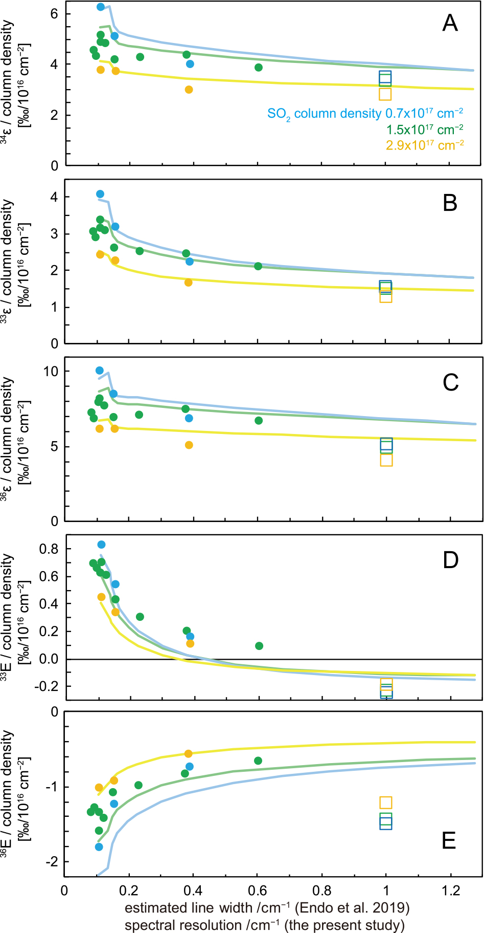
To date, no photolysis experiments have reported fractionation factors under experimental conditions (<1018 cm–2 of column density and ~1 cm–1 of line width) such that the results may be compared with this study. Thus, the total pressure and column density dependence systematically tested by Endo et al. (2019) were extrapolated for comparison with this study. Although some differences exist between spectral resolution and pressure broadened spectra, Fig. 7 shows the slopes of fractionation factors/column density with respect to the SO2 absorption line width at a constant SO2 column density. The absorption line width was assumed to be 1 cm–1, which is equal to the spectral resolution. Meanwhile, the line widths were estimated from pressure broadening, namely, the total atmospheric pressures and a pressure broadening coefficient of SO2 (0.30 ± 0.03 cm–1 atm–1 for N2 atmosphere, Lyons et al., 2018).
In the photolysis experiments conducted by Endo et al. (2019), the total pressure dependence of the 34ε/SO2 column density was relatively small, suggesting that the absorption line width does not strongly affect 34ε (Fig. 7A). This is consistent with the fact that this study (~1 cm–1) reproduced the 34ε/column density of photolysis experiments, despite the unresolved absorption spectra (Fig. 6A and B). On the other hand, this study’s predicted negative 33E/SO2 column density did not match the results of previous experiments (Fig. 6G and H). However, the 33E/column density slope was sensitive to the total pressure and clearly decreased at high total pressure (Fig. 7D). At >0.5 cm–1 of the estimated SO2 absorption line width, a negative 33E/column density was predicted (Fig. 7D, lines), which was consistent with the results of this study. With regards to 33ε and 36ε, the relationship between the SO2 column density (Fig. 6C–F) and absorption line width (Fig. 7B and C) displayed similarities to the 34ε trends; however, they are not as easily reproducible as 34ε. With regard to 36E, this study reproduced results within an approximately 10‰ variation below 5 × 1017 cm2. However, the 36E/SO2 column density slope did not reproduce the broadening model well (Fig. 7E). Consequently, 32,33,34,36SO2 cross-sections may also reproduce 33E/column density when the spectral resolution is improved; however, this is a topic requiring further research. At >1018 cm–2 of SO2 column density, the 34ε in this study is overestimated in comparison to that of photochemical experiments (Fig. 6A). The cause for this is ultimately unclear; however, if a gas with broad absorption spectra exists, the SO2 photolysis rate will decrease at the rear side of the chamber, and the observed fractionations will be smaller than the predicted fractionations of the column density.
Taken together, the 32,33,34,36SO2 absorption spectra reported by this study are likely useful for predicting 34ε during SO2 photolysis at below 1018 cm–2 of SO2 column density. The spectral resolution dependence of the 34ε/SO2 column density is small, and 34ε/SO2 column density of Endo et al. (2015) is similar to that of this study (Fig. 5A). Endo et al. (2015) may be more convenient to utilize than this study, given the availability of 190–220-nm wavelength cross-sections, enhanced precision, and relative ease of calculation due to its low spectral resolution and coarse wavelength steps. Since 33E is sensitive to the SO2 absorption line width, this study could not predict 33E at less than ~1 bar atmospheric pressure, where the absorption line width is less than ~0.3 cm–1 (Fig. 7D). On the contrary, at high atmospheric pressures in which the absorption line width reaches ~1 cm–1, such as in the Venus’ atmosphere, it may be possible to predict 33E (Fig. 7D).
Applying a self-shielding model using the synthesized absorption spectra to laboratory experiments and natural samples
As described in Section “Calculations of self-shielding using synthesized absorption spectra”, in the case of complete discrete absorption spectra of SO2 (Fig. 1A), the self-shielding during SO2 photolysis arises from MIF-S with 33E/34ε and 36E/33E of +0.52 and –1.63, respectively. Interestingly, the slopes are closer to the Archean MIF-S (Δ33S/δ34S ~ +0.9, Δ36S/Δ33S ~ –0.9), than the MIF-S as predicted by the SO2 cross-section of this study (Δ33S/δ34S ~ –0.1, positive Δ36S/Δ33S) and as observed in SO2 photolysis experiments (Δ33S/δ34S ≤ ~ +0.1, Δ36S/Δ33S ≤ ~ –2.4). The observation that the slopes are different from the ideally discrete spectra case implies that the absorption spectra of 32SO2 overlap with those of 33SO2; that is, UV attenuation by 32SO2 absorption decreases not only the 32SO2 photolysis rate constants but also the 33SO2 photolysis rate constants (e.g., Ono, 2017; Endo et al., 2019; Lyons, 2020). Isotope fractionation by self-shielding under the ideal conditions in which absorption lines are narrow can be tested with further laboratory experiments such as SO2 photolysis at low temperature and low pressure and photolysis using a species with a more discrete absorption spectra (e.g., sulfur monoxide (SO), Sarka and Nanbu, 2019).
This simple model predicted that self-shielding leads to large clumped isotope depletion in products and enrichment in reagents (Section “Calculations of self-shielding using synthesized absorption spectra”). Clumped isotopes may possibly be a fingerprint of self-shielding. However, signatures related to self-shielding have not been identified. In the case of SO2 photolysis, S–O clumped isotopes are enriched in residual SO2 and are depleted in the product SO. To preserve the clumped isotope signatures, S–O bonds must remain in the molecules. In laboratory experiments of SO2 photolysis (e.g., Ono et al., 2013), the S–O bonds in the residual SO2 would remain, although the bonds in the produced SO were likely destroyed via SO photolysis. Therefore, an enrichment signature may exist in residual SO2. However, thus far, methods for analyzing S–O clumped isotopes in SO2 have not been developed; it follows that, to test this, sufficient analysis methods must be developed.
Conclusions
We measured the 32SO2, 33SO2, 34SO2, and 36SO2 absorption spectra from 206 to 220 nm at 296 K, set to 1 cm–1 wavelength resolution. The resolution was 25 times higher than has been previously reported. The accuracy was approximately 10%. Compared with previous reports of high-resolution spectra for SO2 at natural abundance, the wavelength appeared to offset from ~0.016 nm, and the magnitudes of the cross-section at the absorption peak wavelength seemed small. However, this had insignificant effects on modeling isotopic self-shielding. Using the measured absorption spectra, we estimated the sulfur isotope fractionation by self-shielding in SO2 photolysis.
This study roughly reproduced the 34ε/(SO2 column density) slope of previous SO2 photolysis experiments; however, the spectral resolution was insufficient to resolve the Doppler widths. This finding likely reflects the insensitivity of 34ε to the absorption line width, which is supported by the total pressure effect observed in previous SO2 photolysis experiments. The second key characteristic of the prediction was the negative 33E/(SO2 column density) slope. This did not match previous photolysis experiments, but was consistent with prior observations that the slopes were smaller in SO2 photolysis experiments at higher total pressures. Under a high pSO2 atmosphere, strong self-shielding and strong pressure broadening should occur. This provides the basis for the novel suggestion that spectroscopic research may be linked to photolysis experiments with MIF-S.
Additionally, we modeled an ideal case in which the absorption lines are narrow below the Doppler width. The produced self-shielding originates from MIF-S closer to the Archean trend than described in previous photolysis experiments and spectroscopic measurements. This suggests that self-shielding remains a major candidate for MIF-S in the Archean atmosphere.
Acknowledgments
We would like to thank Shohei Hattori and Naohiro Yoshida for sample preparation and Matthew S. Johnson for technical advice. We also thank James Lyons and an anonymous reviewer for their constructive comments. The editor, Tsubasa Otake, provided advice on the organization of the paper. Cross-sections of 32,33,34,36SO2 reported by Lyons (2007) were provided by James Lyons. This research was funded by JSPS KAKENHI (grant numbers JP16J06990, JP17H06105, JP20H01975, JP20K14593, and 24740364). The authors would also like to thank Editage (www.editage.com) for English language editing.
References
- Avice, G., Marty, B., Burgess, R., Hofmann, A., Philippot, P., Zahnle, K. and Zakharov, D. (2018) Evolution of atmospheric xenon and other noble gases inferred from Archean to Paleoproterozoic rocks. Geochim. Cosmochim. Acta 232, 82–100.
- Babikov, D. (2017) Recombination reactions as a possible mechanism of mass-independent fractionation of sulfur isotopes in the Archean atmosphere of Earth. Proc. Natl Acad. Sci. USA 114, 3062–3067.
- Ball, C. D., Dutta, J. M., Goyette, T. M., Helminger, P. and De Lucia, F. C. (1996) The pressure broadening of SO2 by N2, O2, He, and H2 between 90 and 500 K. J. Quant. Spectrosc. Radiat Transf. 56, 109–117.
- Blackie, D., Blackwell‐Whitehead, R., Stark, G., Pickering, J. C., Smith, P. L., Rufus, J. and Thorne, A. P. (2011) High‐resolution photoabsorption cross‐section measurements of SO2 at 198 K from 213 to 325 nm. J. Geophys. Res. 116, E03006.
- Cazzoli, G. and Puzzarini, C. (2012) N2-, O2-, H2-, and He-broadening of SO2 rotational lines in the mm-/submm-wave and THz frequency regions: The J and Ka dependence. J. Quant. Spectrosc. Radiat. Transf. 113, 1051–1057.
- Chakraborty, S., Ahmed, M., Jackson, T. L. and Thiemens, M. H. (2008) Experimental test of self-shielding in vacuum ultraviolet photodissociation of CO. Science 321, 1328–1331.
- Chakraborty, S., Muskatel, B. H., Jackson, T. L., Ahmed, M., Levine, R. D. and Thiemens, M. H. (2014) Massive isotopic effect in vacuum UV photodissociation of N2 and implications for meteorite data. Proc. Natl. Acad. Sci. USA 111, 14704–14709.
- Claire, M. W., Kasting, J. F., Domagal-Goldman, S. D., Stüeken, E. E., Buick, R. and Meadows, V. S. (2014) Modeling the signature of sulfur mass-independent fractionation produced in the Archean atmosphere. Geochim. Cosmochim. Acta 141, 365–380.
- Danielache, S. O., Eskebjerg, C., Johnson, M. S., Ueno, Y. and Yoshida, N. (2008) High-precision spectroscopy of 32S, 33S, and 34S sulfur dioxide: Ultraviolet absorption cross sections and isotope effects. J. Geophys. Res. 113, D17314.
- Danielache, S. O., Hattori, S., Johnson, M. S., Ueno, Y., Nanbu, S. and Yoshida, N. (2012) Photoabsorption cross-section measurements of 32S, 33S, 34S, and 36S sulfur dioxide for the B1B1-X1A1 absorption band. J. Geophys. Res. 117, D24301.
- Eiler, J. M. (2007) “Clumped-isotope” geochemistry—The study of naturally-occurring, multiply-substituted isotopologues. Earth Planet. Sci. Lett. 262, 309–327.
- Endo, Y., Danielache, S. O., Ueno, Y., Hattori, S., Johnson, M. S., Yoshida, N. and Kjaergaard, H. G. (2015) Photoabsorption cross-section measurements of 32S, 33S, 34S, and 36S sulfur dioxide from 190 to 220 nm. J. Geophys. Res. Atmos. 120, 2546–2557.
- Endo, Y., Ueno, Y., Aoyama, S. and Danielache, S. O. (2016) Sulfur isotope fractionation by broadband UV radiation to optically thin SO2 under reducing atmosphere. Earth Planet. Sci. Lett. 453, 9–22.
- Endo, Y., Danielache, S. O. and Ueno, Y. (2019) Total pressure dependence of sulfur mass-independent fractionation by SO2 photolysis. Geophys. Res. Lett. 46, 483–491.
- Farquhar, J. (2018) Sulfur Isotopes. Encyclopedia of Geochemistry. Encyclopedia of Earth Sciences Series (White M. W. ed.), Springer, Cham. https://doi.org/10.1007/978-3-319-39193-9_74-1
- Farquhar, J., Bao, H. and Thiemens, M. (2000a) Atmospheric influence of Earth’s earliest sulfur cycle. Science 289, 756–759.
- Farquhar, J., Savarino, J., Jackson, T. L. and Thiemens, M. H. (2000b) Evidence of atmospheric sulphur in the martian regolith from sulphur isotopes in meteorites. Nature 404, 50–52.
- Farquhar, J., Savarino, J., Airieau, S. and Thiemens, M. H. (2001) Observation of wavelength-sensitive mass-independent sulfur isotope effects during SO2 photolysis: Implications for the early atmosphere. J. Geophys. Res. 106, 32829–32839.
- Feaga, L. M., McGrath, M. and Feldman, P. D. (2009) Io’s dayside SO2 atmosphere. Icarus 201, 570–584.
- Franz, H. B., Danielache, S. O., Farquhar, J. and Wing, B. A. (2013) Mass-independent fractionation of sulfur isotopes during broadband SO2 photolysis: Comparison between 16O- and 18O-rich SO2. Chem. Geol. 362, 56–65.
- Freeman, D. E., Yoshino, K., Esmond, J. R., and Parkinson, W. H. (1984) High resolution absorption cross section measurements of SO2 at 213 K in the wavelength region 172–240 nm. Planet. Space Sci. 32, 1125–1134.
- Gaillard, F., Scaillet, B. and Arndt, N. T. (2011) Atmospheric oxygenation caused by a change in volcanic degassing pressure. Nature 478, 229–232.
- Gordon, I. E., Rothman, L. S., Hill, C., Kochanov, R. V., Tan, Y., Bernath, P. F., Birk, M., Boudon, V., Campargue, A., Chance, K. V., Drouin, B. J., Flaud, J. -M., Gamache, R. R., Hodges, J. T., Jacquemart, D., Perevalov, V. I., Perrin, A., Shine, K. P., Smith, M. -A. H., Tennyson, J., Toon, G. C., Tran, H., Tyuterev, V. G., Barbe, A., Császár, A. G., Devi, V. M., Furtenbacher, T., Harrison, J. J., Hartmann, J. -M., Jolly, A., Johnson, T. J., Karman, T., Kleiner, I., Kyuberis, A. A., Loos, J., Lyulin, O. M., Massie, S. T., Mikhailenko, S. N., Moazzen-Ahmadi, N., Müller, H. S. P., Naumenko, O. V., Nikitin, A. V., Polyansky, O. L., Rey, M., Rotger, M., Sharpe, S. W., Sung, K., Starikova, E., Tashkun, S. A., Auwera, J. V., Wagner, G., Wilzewski, J., Wcisło, P., Yu, S. and Zak, E. J. (2017) The HITRAN2016 molecular spectroscopic database. J. Quant. Spectrosc. Radiat. Transf. 203, 3–69.
- Halevy, I., Zuber, M. T. and Schrag, D. P. (2007) A sulfur dioxide climate feedback on early Mars. Science 318, 1903–1907.
- Harris, E., Sinha, B., Hoppe, P., Crowley, J. N., Ono, S. and Foley, S. (2012) Sulfur isotope fractionation during oxidation of sulfur dioxide: gas-phase oxidation by OH radicals and aqueous oxidation by H2O2, O3 and iron catalysis. Atmos. Chem. Phys. 12, 407–423.
- Harman, C. E., Pavlov, A. A., Babikov, D. and Kasting, J. F. (2018) Chain formation as a mechanism for mass‐independent fractionation of sulfur isotopes in the Archean atmosphere. Earth Planet. Sci. Lett. 496, 238–247.
- Heicklen, J., Kelly, N. and Partymiller, K. (1980) The photophysics and photochemistry of SO2. Rev. Chem. Intermed. 3, 315–404.
- Hermans, C., Vandaele, A. C. and Fally, S. (2009) Fourier transform measurements of SO2 absorption cross sections: I. Temperature dependence in the 24 000–29 000 cm–1 (345–420 nm) region, J. Quant. Spectrosc. Radiat. Transf. 110, 756–765.
- Holland, H. D. (2002) Volcanic gases, black smokers, and the great oxidation event. Geochim. Cosmochim. Acta 66, 3811–3826.
- Ignatiev, A. V., Velivetskaya, T. A. and Yakovenko, V. V. (2019) Effect of mass-independent isotope fractionation of sulfur (Δ33S and Δ36S) during SO2 photolysis in experiments with a broadband light source. Geochemistry Int. 57, 751–760.
- Izon, G., Zerkle, A. L., Williford, K. H., Farquhar, J., Poulton, S. W. and Claire, M. W. (2017) Biological regulation of atmospheric chemistry en route to planetary oxygenation. Proc. Natl. Acad. Sci. USA 114, E2571–E2579.
- Johnson, S. S., Mischna, M. A., Grove, T. L. and Zuber, M. T. (2008) Sulfur-induced greenhouse warming on early Mars. J. Geophys. Res. 113, E08005.
- Katagiri, H., Sako, T., Hishikawa, A., Yazaki, T., Onda, K., Yamanouchi, K. and Yoshino, K. (1997) Experimental and theoretical exploration of photodissociation of SO2 via the 1B2 state: identification of the dissociation pathway. J. Mol. Struct. 413–414, 589–614.
- Koplow, J. P., Kliner, D. A. V. and Goldberg, L. (1998) Development of a narrow‐band, tunable, frequency‐quadrupled diode laser for UV absorption spectroscopy. Appl. Opt. 37, 3954–3960.
- Kroll, J. A., Frandsen, B. N., Rapf, R. J., Kjaergaard, H. G. and Vaida, V. (2018) Reactivity of electronically excited SO2 with alkanes. J. Phys. Chem. A 122, 7782–7789.
- Kühnemann, F., Heiner, Y., Sumpf, B. and Herrmann, Ka. (1992) Line broadening in the ν3 band of SO2: Studied with diode laser spectroscopy. J. Mol. Spectrosc. 152, 1–12.
- Lin, M. and Thiemens, M. H. (2020) A simple elemental sulfur reduction method for isotopic analysis and pilot experimental tests of symmetry-dependent sulfur isotope effects in planetary processes. Geochem. Geophys. Geosyst. 21, e2020GC009051.
- Lyons, J. R. (2007) Mass-independent fractionation of sulfur isotopes by isotope-selective photodissociation of SO2. Geophys. Res. Lett. 34, L22811.
- Lyons, J. R. (2020) An analytical formulation of isotope fractionation due to self-shielding. Geochim. Cosmochim. Acta 282, 177–200.
- Lyons, J. R., Herde, H., Stark, G., Blackie, D. S., Pickering, J. C. and de Oliveira, N. (2018) VUV pressure-broadening in sulfur dioxide. J. Quant. Spectrosc. Radiat. Transf. 210, 156–164.
- Masterson, A. L., Farquhar, J. and Wing, B. A. (2011) Sulfur mass-independent fractionation patterns in the broadband UV photolysis of sulfur dioxide: Pressure and third body effects. Earth Planet. Sci. Lett. 306, 253–260.
- Miller, C. E. and Yung, Y. L. (2000) Photo-induced isotopic fractionation. J. Geophys. Res. 105, 29039–29051.
- Mishima, K., Yamazaki, R., Satish-Kumar, M., Ueno, Y., Hokada, T. and Toyoshima, T. (2017) Multiple sulfur isotope geochemistry of Dharwar Supergroup, Southern India: Late Archean record of changing atmospheric chemistry. Earth Planet. Sci. Lett. 464, 69–83.
- Ohmoto, H. (2020) A seawater-sulfate origin for early Earth’s volcanic sulfur. Nature Geosci. 13, 576–583.
- Okabe, H. (1971) Fluorescence and predissociation of sulfur dioxide. J. Am. Chem. Soc. 93, 7095–7096.
- Olson, S. L., Ostrander, C. M., Gregory, D. D., Roy, M., Anbar, A. D. and Lyons, T. W. (2019) Volcanically modulated pyrite burial and ocean–atmosphere oxidation. Earth Planet. Sci. Lett. 506, 417–427.
- Okazaki, A., Ebata, T., and Mikami, N. (1997) Degenerate four-wave mixing and photofragment yield spectroscopic study of jet-cooled SO2 in the C1B2 state: Internal conversion followed by dissociation in the X state. J. Chem. Phys. 107, 8752–8758.
- Ono, S. (2017) Photochemistry of sulfur dioxide and the origin of mass-independent isotope fractionation in Earth’s atmosphere. Annu. Rev. Earth Planet. Sci. 45, 301–329.
- Ono, S., Kaufman, A. J., Farquhar, J., Sumner, D. Y. and Beukes, N. J. (2009) Lithofacies control on multiple-sulfur isotope records and Neoarchean sulfur cycles. Precambrian Res. 169, 58–67.
- Ono, S., Whitehill, A. R. and Lyons, J. R. (2013) Contribution of isotopologue self-shielding to sulfur mass-independent fractionation during sulfur dioxide photolysis. J. Geophys. Res. Atmos. 118, 2444–2454.
- Pavlov, A. A. and Kasting, J. F. (2002) Mass-independent fractionation of sulfur isotopes in Archean sediments: Strong evidence for an anoxic Archean atmosphere. Astrobiology 2, 27–41.
- Ran, H., Xie, D. and Guo, H. (2007) Theoretical studies of equation C̃ 1B2 absorption spectra of SO2 isotopomers. Chem. Phys. Lett. 439, 280–283.
- Romero, A. B. and Thiemens, M. H. (2003) Mass-independent sulfur isotopic compositions in present-day sulfate aerosols. J. Geophys. Res. Atmos. 108, 4524.
- Rufus, J., Stark, G., Smith, P. L., Pickering, J. C. and Thorne, A. P. (2003) High-resolution photoabsorption cross-section measurements of SO2, 2: 220 to 325 nm at 295 K. J. Geophys. Res. 108, 5011.
- Rufus, J., Stark, G., Thorne, A. P., Pickering, J. C., Blackwell-Whitehead, R. J., Blackie, D. and Smith, P.L. (2009) High-resolution photoabsorption cross-section measurements of SO2 at 160 K between 199 and 220 nm. J. Geophys. Res. 114, E06003.
- Sarka, K. and Nanbu, S. (2019) Total absorption cross section for UV excitation of sulfur monoxide. J. Phys. Chem. A 123, 3697–3702.
- Savarino, J., Romero, A., Cole-Dai, J., Bekki, S. and Thiemens, M. H. (2003) UV induced mass-independent sulfur isotope fractionation in stratospheric volcanic sulfate. Geophys. Res. Lett. 30, 2131.
- Stark, G., Smith, P. L., Rufus, J., Thorne, A. P., Pickering, J. C. and Cox, G. (1999) High-resolution photoabsorption cross-section measurements of SO2 at 295 K between 198 and 220 nm. J. Geophys. Res. 104, 16585–16590.
- Sumpf, B., Fleischmann, O. and Kronfeldt, H. -D. (1996a) Self-, air-, and nitrogen-broadening in the v1 band of SO2. J. Mol. Spectrosc. 176, 127–132.
- Sumpf, B., Schöne, M. and Kronfeldt, H. -D. (1996b) Self- and air-broadening in the v3 band of SO2. J. Mol. Spectrosc. 179, 137–141.
- Sumpf, B. (1997) Experimental investigation of the self-broadening coefficients in the v1 + v3 band of SO2 and the 2v2 band of H2S. J. Mol. Spectrosc. 181, 160–167.
- Tasinato, N., Charmet, A. P., Stoppa, P., Giorgianni, S. and Buffa, G. (2010) Spectroscopic measurements of SO2 line parameters in the 9.2 μm atmospheric region and theoretical determination of self-broadening coefficients. J. Chem. Phys. 132, 044315.
- Tasinato, N., Charmet, A. P., Stoppa, P., Buffa, G. and Puzzarini, C. (2013) A complete listing of sulfur dioxide self-broadening coefficients for atmospheric applications by coupling infrared and microwave spectroscopy to semiclassical calculations. J. Quant. Spectrosc. Radiat. Transf. 130, 233–248.
- Tasinato, N., Charmet, A. P., Stoppa, P., Giorgianni, S. and Buffa, G. (2014) N2-, O2-and He-collision-induced broadening of sulfur dioxide ro-vibrational lines in the 9.2 μm atmospheric window. Spectrochim. Acta A 118, 373–379.
- Thiemens, M. H. and Lin, M. (2021) Discoveries of mass independent isotope effects in the solar system: Past, present and future. Rev. Mineral. Geochem. 86, 35–95.
- Tokue, I. and Nanbu, S. (2010) Theoretical studies of absorption cross sections for the C̃ 1B2‐X̃ 1A1 system of sulfur dioxide and isotope effects. J. Chem. Phys. 132, 024301.
- Ueno, Y., Johnson, M. S., Danielache, S. O., Eskebjerg, C., Pandey, A. and Yoshida, N. (2009) Geological sulfur isotopes indicate elevated OCS in the Archean atmosphere, solving faint young sun paradox. Proc. Natl. Acad. Sci. USA 106, 14784–14789.
- Vandaele, A. C., Simon, P. C., Guilmot, J. M., Carleer, M. and Colin, R. (1994) SO2 absorption cross section measuring in the UV using a Fourier transform spectrometer. J. Geophys. Res. Atoms. 99, 25599–25605.
- Vandaele, A. C., Hermans, C. and Fally, S. (2009) Fourier transform measurements of SO2 absorption cross sections: II. Temperature dependence in the 29 000–44 000 cm–1 (227–345 nm) region. J. Quant. Spectrosc. Radiat. Transf. 110, 2115–2126.
- Vandaele, A. C., Korablev, O., Belyaev, D., Chamberlain, S., Evdokimova, D., Encrenaz, Th., Esposito, L., Jessup, K. L., Lefèvre, F., Limaye, S., Mahieux, A., Marcq, E., Mills, F. P., Montmessin, F., Parkinson, C. D., Robert, S., Roman, T., Sandor, B., Stolzenbach, A., Wilson, C. and Wilquet, V. (2017) Sulfur dioxide in the Venus atmosphere: I. Vertical distribution and variability. Icarus 295, 16–33.
- Wang, D. T., Welander, P. V. and Ono, S. (2016) Fractionation of the methane isotopologues 13CH4, 12CH3D, and 13CH3D during aerobic oxidation of methane by Methylococcus capsulatus (Bath). Geochim. Cosmochim. Acta 192, 186–202.
- Whitehill, A. R. and Ono, S. (2012) Excitation band dependence of sulfur isotope mass-independent fractionation during photochemistry of sulfur dioxide using broadband light sources. Geochim. Cosmochim. Acta 94, 238–253.
- Whitehill, A. R., Xie, C., Hu, X., Xie, D., Guo, H. and Ono, S. (2013) Vibronic origin of sulfur mass-independent isotope effect in photoexcitation of SO2 and the implications to the early Earth’s atmosphere. Proc. Natl. Acad. Sci. USA 110, 17697–17702.
- Whitehill, A. R., Jiang, B., Guo, H. and Ono, S. (2015) SO2 photolysis as a source for sulfur mass-independent isotope signatures in stratospheric aerosols. Atmos. Chem. Phys. 15, 1843–1864.
- Whitehill, A. R., Joelsson, L. M. T., Schmidt, J. A., Wang, D. T., Johnson, M. S. and Ono, S. (2017) Clumped isotope effects during OH and Cl oxidation of methane. Geochim. Cosmochim. Acta 196, 307–325.
- Wu, C. Y. R., Yang, B. W., Chen, F. Z., Judge, D. L., Caldwell, J. and Trafton, L. M. (2000) Measurements of high‐, room‐, and low‐temperature photoabsorption cross sections of SO2 in the 2080‐ to 2950‐Å region, with application to Io. Icarus 145, 289–296.
- Yeung, L. Y., Li, S., Kohl, I. E., Haslun, J. A., Ostrom, N. E., Hu, H., Fischer, T. P., Schauble, E. A. and Young, E. D. (2017) Extreme enrichment in atmospheric 15N15N. Sci. Adv. 3, eaao6741.
- Zahnle, K., Claire, M. and Catling, D. (2006) The loss of mass-independent fractionation in sulfur due to a Palaeoproterozoic collapse of atmospheric methane. Geobiology 4, 271–283.
- Zahnle, K. J., Gacesa, M. and Catling, D. C. (2019) Strange messenger: A new history of hydrogen on Earth, as told by Xenon. Geochim. Cosmochim. Acta 244, 56–85.
- Zerkle, A. L., Claire, M. W., Domagal-Goldman, S. D., Farquhar, J. and Poulton, S. W. (2012) A bistable organic-rich atmosphere on the Neoarchaean Earth. Nat. Geosci. 5, 359–363.