Abstract
The amount, chemical composition and distribution of nonmetallic inclusions are important factors when determining steel quality. Therefore, in recent years, a great deal of effort has gone into developing robust detection systems for nonmetallic inclusions. Various methods have been suggested, but most of them require extensive sample preparation. As a result, these methods are only suitable for analyzing micro-inclusions. For estimating the macrocleanliness, these methods are too slow because, due to the rarity of these kinds of inclusions, huge sample volumes are needed. To overcome this problem, we propose a new detection methodology that can detect inclusions and defects, like microcracks and shrinkage holes, at a range of between 5 μm and several thousands of a μm. At the same time, it is fast enough to process samples of very large steel volumes of 300 × 120 × 90 mm³ in size. Similar to the classic metallographic approach using a microscope and polished steel surfaces, the steel surface of a sample is recorded by a moving CCD sensor with a pixel size of 2.75 μm. Inclusions are detected using image processing techniques. Then, the steel surface is milled off, removing a 10 μm chip, and the recording step is repeated. Processing the whole sample in this way allows us to reconstruct the three-dimensional shape of inclusions and other defects and gives us information about the spatial distribution of these inclusions. In this paper, we describe this system in greater detail and describe the initial results of our approach.
1. Introduction
Non-metallic inclusions have a major impact on the mechanical properties and therefore on the quality of steel.1) Several sources of these inclusions have recently been identified. While some inclusions form shortly after the deoxidant is added to the liquid steel or while the steel is cooling to its liquidus temperature,2) others result from contaminations added during the production process. But inclusions differ not only in their source and time of formation, but also in their size,3) morphology4,5) and chemical composition.6) A wide range of inclusions have been observed, from those smaller than 5 μm (micro-inclusions) to those larger than 100 μm (macro-inclusions). Typical shapes, that are reported in the literature, are globular inclusions, which have a nearly spherical form, and dendritic inclusions, which have sharp edges and corners. This difference in shape results from different formation processes and is an indicator of a different chemical composition.4,5) Analyzing this morphology aids understanding of the formation process and provides the opportunity to optimize the production process so that fewer inclusions remain in the product. In recent years various techniques for detecting and analyzing inclusions have been proposed.7) Some of them have been standardized in the form of norms and are used in industry. They differ in detail from country to country, but the general procedure is the same. In a polished steel surface larger than 160 mm², inclusions are detected with a microscope (using image processing or manual inspection) and rated according to their size and morphology.8,13) While this method can reveal two-dimensional shapes and is suitable for analyzing microcleanliness, the sample size is too small for analyzing macrocleanliness. An alternative technique that attempts to overcome these problems is MIDAS.9,10,11,12) Using ultrasonic sound to detect inclusions in specially prepared steel samples (so-called “surfboard” samples), this approach is capable of processing very large steel volumes to give a significant measure of the macrocleanliness. On the other hand, due to the deformation of the samples and the detection methodology, this approach reveals no information about the morphology. Furthermore, an analysis of the micro cleanliness is not possible due to the resolution of the sensor.
To overcome these problems, we propose a new system which seeks to combine the advantages of MIDAS with the classic approach using an optical system. In our approach, a steel sample of a maximum of 300 × 120 × 90 mm³ cut directly from the continuous caster is mounted on a linear positioning system. The surface can be recorded by a moving CCD sensor with a pixel size of 2.75 μm. The small digitalized image patches are stitched into one large gigapixel image and inclusions and other kind of defects are segmented automatically in this image. The segmented defects can be characterized by their two dimensional shape, and the size distribution can be estimated for the entire steel volume stereologically. If a further chemical analysis is desired, it is possible to ask the system for a map with interesting inclusions, which can be selectively processed by a laser-induced breakdown spectroscopy system (LIBS),21,22) or a microscope optic. To give a better approximation of the cleanliness and to reconstruct the three-dimensional morphology, in the next processing step the steel surface is milled off, removing a 10 μm chip, and the image recording step is repeated. By repeating this process several times, we are able to create a virtualized three-dimensional image of the entire steel volume. This allows us to analyze the spatial distribution of inclusions and defects in general, classify them according to their three-dimensional shape and visualize them using real-time rendering methods. Below, we will discuss our system in greater detail and present our initial results.
2. System Overview
Our system is designed after the pipes and filters pattern. Each component in this pipeline uses the results from the previous pipeline stage as an input parameter, transforms the data and passes them to the next step. If one stage is not yet ready for new input parameters, data are cached in a queue. This permits parallel and autonomous operation of each component and ensures a high throughput. The first component is the image recording unit (Section 3), which records the image and passes it to the image processing unit (Section 4). The image processing unit identifies possible defects, like inclusions, cracks or shrinkage holes, and passes this information along with the raw data about each recognized defect to the morphological analysis unit (Section 5). In this way, the process data are heavily reduced from an image with a possible size of several gigabytes to a data stream consisting only of defect pixels. At this point in the pipeline, the mill is triggered to mill off a new slice of the sample. The morphological analysis unit traces the defects through the steel slices and tries to detect if a defect has been completely milled off. To do this, it has to cache defect data from the previous layers. As soon as a defect is detected as complete (i.e., the defect can finally be reconstructed in its entirety), certain shape parameters are calculated and the defect is classified. In the current state of our system, we have identified parameters to distinguish between cracks, non-metallic inclusions, entrapped gas bubbles and artifacts. Artifacts result from the periodic milling pattern; they are created by the heavy mechanical stresses involved in the milling process. They may be detected at this point in the process because they were not filtered out properly by the image processing unit. Every unit up to this point can send a stop request to the mill. This is especially useful when an interesting structure is detected on the surface and the mill should be prevented from milling it off, so that a deeper investigation using LIBS or a microscope optic can be performed. Another reason for stopping the mill is that, when enough slices have been milled off to give a statistically significant measure of the steel quality, it is advisable to stop the mill in order to save time and to prevent the indexable change from deteriorating. Of course, the system operator can also stop the process manually at any time. Finally, after classification by the morphological analysis unit, the raw data together with all the calculated parameters of the complete defects are continuously written to the file system. We use the HDF5 file format, a general purpose format for storing large binary data from scientific applications. Doing so increases the interoperability of our system because HDF5 is supported by many software packages, such as MATLAB, R and Mathematica, and we are able to use these products for more complex data analysis tasks. We also use the HDF5 file to load the raw data for rendering defects in real time (Section 6). In addition, we write all defect metadata, calculated by the morphological analysis unit, into a relational database. This simplifies access to the data for web servers and permits a quick overview of the sample information via web browser. In the following sections, we describe the stages of the processing pipeline in more detail.
3. Image Recording
For image capture we use an 8-megapixel CCD sensor from Kodak with a pixel pitch of 5.5 μm. Both the camera and the steel sample are positioned by a Cartesian xyz robot. The robot is split into an x-axis and a combined y/z-axis, which is placed onto a portal directly above the x-axis. The camera, optics and lighting are mounted onto the z-axis and are flexibly fixed by an optical rail. For accurate step-by-step positioning of the camera, we decided to use crossed-roller bearing stages for the y/z-axis. For best smoothness characteristics in scanning mode, the x-axis is an air-bearing linear stage (See Fig. 1 for an image of our system). We split the positioning system this way so that the camera does not have to move in scanning mode, which avoids vibrations during image capture. While capturing images, only the x-axis, which holds the steel sample, moves. Every axis has a calibrated bi-directional repeatability better than 1 μm, and its smallest step size is 10 nm. Since we want to capture the entire steel surface with a pixel size of 2.75 μm, the repeatability is so accurate that misplacements will not be recognizable in the final image. However, even at magnifications of up to 600 nm per pixel, there will be a two-pixel displacement at most. Finally, the x-axis has a travel range of 400 mm, the y-axis 110 mm and the z-axis 40 mm, which is for focusing the camera.

We currently use geometrically distortion-free macro lenses with only small magnification factors up to 2.5x. For the initial implementation of our scanning system we did not choose microscope lenses with higher magnifications and better optical resolutions, because a macro lens has a greater depth of field, which, in our case, is 40 μm, compared to the very shallow depth of field of microscope lenses, which is usually 5 μm or less. Since we are scanning large surfaces, we favored the larger depth of field in order to avoid any need for focus stacking, which results in longer image recording times. For focusing, we implemented a straightforward image processing algorithm based on Sobel filtering of the video image.
Lighting the steel surface is very challenging because the milling grooves cause harsh shadows on the otherwise highly reflective surface. To avoid most of these shadows under brightfield illumination, we use coaxial lighting comprising a diffusor plate and a dichroic half-mirror, which allows better light throughput than other half-mirrors. We place this coaxial lighting module within the free working distance between the surface and the lens instead of using inline illumination, in which case it would be placed between the fore lens and the camera or other tube lenses. This is because the diffuse light source should be placed as close to the surface as possible so that, after passing the diffusor, the light is not redirected when passing the fore lens. Under brightfield illumination, anomalies like nonmetallic inclusions, microcracks or shrinkage holes appear dark in the image since, because of their roughness properties, they do not directly reflect light back into the fore lens. This is sufficient for optically recognizing their shapes, sizes, centroids and overall distribution. Image capture is also very fast because exposure times are in the range of microseconds; this is because the uninteresting background (the clean steel matrix) reflects a great deal of light; only the anomalies do not. On the other hand, we could not tell much about the inner texture of a nonmetallic inclusion or their spectral properties if we only used brightfield illumination. Therefore, for further characterization darkfield illumination is essential, where most of the scattering light is due to the nonmetallic inclusions and less to none is reflected by the steel surface. Here, the anomalies appear bright in the image, and the clean steel matrix is ideally black. Under this lighting setup, much less light is reflected into the camera optics, requiring much longer exposure times, as much as a few hundred milliseconds. For this type of illumination we use a darkfield ring light with an additional diffusor.
Two types of application are currently supported: a high-speed scanning mode with coarser resolution under brightfield illumination for fast capture of volumetric slices and a slower high-resolution step-by-step image capture under darkfield illumination for analyzing single surfaces. In scanning mode, the probe is continuously moved under the camera and image capture is triggered directly by the controller of the moving axis so that the camera is synchronized with the position of the probe. We achieve a scanning speed of 50 mm/s; thus, the surface of a standard steel probe of 300 × 120 mm2 is recorded within 30 seconds. The resolution is downsampled to a pixel size of 20 μm, whereas finer resolutions would result in longer exposure times, thus creating motion blur. This is a compromise between resolution and scanning speed in order to be able to scan hundreds of slices of a steel sample within only several hours. In this way, we can provide real-time statistics about the existence and distribution of larger nonmetallic inclusions, argon bubbles, shrinkage holes and/or cracks.
In another scenario, we capture still images by moving the x-axis in a step-and-settle fashion, whereby images are stitched one after another into a single gigapixel image of the surface. The camera is manually aligned into its orthogonal position with respect to all axes so that no further image processing is needed for image alignment. The manual alignment results in a misplacement of pixels at the transition between two image tiles along both x- and y-axes; this misplacement is usually smaller than 30 μm. Due to the step-and-settle approach and the darkfield illumination, image recording takes much longer: about 15 minutes per surface. However, we achieve images with a pixel size of 2.75 μm, and, by stitching 11 × 23 = 253 still images, we come up with a 4-gigapixel image with which we can analyze the whole 300 × 120 mm² surface area of a standard steel sample at reasonably high resolution. Furthermore, the darkfield illumination gives us rich information about the texture of the detected anomalies.
The metrology system presented here is designed for easy replacement of optics, image sensors and lighting. For example, after a high-resolution gigapixel image of the surface has been recorded, we are able to replace the macro lens with a microscope lens of higher resolution, but lower field of view and shallower depth of field, in only a few steps, because the mounting interface is an optical rail that can be easily reconfigured. After calibrating the new mounting position of the microscope lens with respect to the previously captured surface image, we can interactively make new images revealing more details than the gigapixel image for only the most interesting observations, which have already been automatically extracted through image analysis. This is another operating mode for the metrology system—interactive exploration.
4. Image Processing
The image processing unit is a central component of our measurement system since all further analyses rely on the quality of the image processing results. The following section describes it in greater detail. Additionally it describes how results from the image processing step can be used to adapt parameters during image recording in order to enhance image quality or detect when the mill’s indexable insert needs to be changed.
4.1. Segmentation of Surface Defects
The images of the milled steel surfaces show a quasiperiodic pattern resulting from the complex interplay of the turning inserts of the milling head with the steel and possible inclusion materials. Within this pattern, small regions showing sections of nonmetallic inclusions, cracks and shrink holes appear. The steel surface is highly reflective and the intensity values of the milling pattern may cover the entire dynamic range of the image sensor. Therefore, simple thresholding methods fail to detect defective regions. On the other hand, rapid processing of each surface layer is needed in order to achieve a high throughput for the whole measurement system.
The regularity of the milling pattern can be analyzed using filters based on the two-dimensional Fourier transform. Aiger and Talbot14) introduced the phase-only transform (PHOT), which detects defects in surface textures. It is based on simple magnitude normalization in the 2D Fourier domain which preserves only the phase information of the image. The PHOT removes all regularities at any scale and indicates small defects with high evidence values, which can simply be thresholded. In the case of brightfield illumination, defects appear dark; thus, only negative evidence values are considered. Using darkfield illumination, objects appear lighter and only positive evidence values are interesting. As larger defects may be recognized with holes, a morphological closing filter is applied to fill any holes. Figure 2 shows example applications of the PHOT on images captured with different illuminations and resolutions.

The PHOT effectively localizes all defective areas and provides precise, shape-preserving segmentation. It mostly relies on the 2D Fourier transform, which is available as speeded up fast Fourier transform (FFT) in many image-processing libraries. To achieve a processing time of less than three seconds per layer with 100 megapixels and meet the high throughput requirements for the entire process, we use high-performance graphics processing units (GPU) for the image-segmentation process.
4.2. Filtering Using Neighboring Layers
Due to the milling process, it is possible for irregular patterns as well as oil drops or metal shavings to appear on the surface. As these artifacts are not relevant to the steel quality, we filter them out using neighboring layers. Since all relevant defects, like nonmetallic inclusions, cracks or shrinkage holes, have a three-dimensional extent, the sections of objects appear on several consecutive images. On the other hand, the objects may change in size and shape, depending on which layer along the z-axis is examined. We use a mathematical dilation operation on the segmentation of each layer to model the changing shape. Finally, a set of dilated layers in a symmetrical neighborhood around every layer is multiplied pixelwise to obtain a weighting layer for the segmentation of each layer. Analyzing surface images with a coarse resolution, we use three neighboring layers for this filtering process, which leads to a minimal detectable object size of 30 μm along the volumetric axis.
4.3. Image-based Process Parameter Adaptation
Our measurement process requires a highly adaptive system to achieve a high degree of automation and, ultimately, cost effectiveness. We use the image data to analyze and adapt important process parameters. The hardness of the steel and the unknown hardness of possible inclusions cause the turning inserts of the milling head to erode rapidly. These have to be replaced regularly because the contrast of the defects to the milling pattern would otherwise be reduced. In order to detect a necessary tool change, we derive four image features: the means and standard deviations of the gray values and low frequencies of the 2D Fourier magnitude spectrum. These features are used to train a multilayer perceptron (MLP) with an assumed wear function of 1100 surface layers. Figure 3 depicts the resulting network output compared to the expected function. Furthermore, we use the average gray value to control the brightness of the lighting system. This is necessary because the reflectance of the steel surface and the resulting amount of light captured by the camera varied greatly. In doing so, we prevent under- or overexposed images that would cause a huge loss of information about defective objects.

5. Morphological Analysis
With the segmented defects in the two-dimensional cut image, continuous slicing of the steel sample allows us to reconstruct the three-dimensional shape of every defect detected by our system. To accomplish this task, the morphological analysis unit caches the segmentation data for every defect as long as the particular defect is not completely milled off. Afterwards, distinguishable shape descriptors are calculated for every defect, so that an online classification of the defects can be carried out parallel to the milling process. Below, we describe how we implemented the reconstruction, which shape descriptors have proven useful and how the classification is done. We start by describing the reconstruction.
5.1. Reconstruction
The input parameter of the morphological analysis unit is a list of pixels that were detected as belonging to defects in the image-processing step. These pixels are treated from now on as volumetric pixels (voxels), i.e., cells on a cuboidal lattice where the lattice distance in x- and y-direction is equal to the pixel size of the camera, and the spacing in z-direction is equal to the chip removal size of the mill. The z-index for a voxel is equal to the number of the current cut images, starting with 0 for the first image. To detect the individual defects in the data, we need a formal definition of the term defect.
We define a defect as a connected voxel set V. A voxel set is called connected if any two points (xa, ya, za), (xb, yb, zb)∈V can be joined by a path which completely lies in V. A path consists of n + 1 points Pi = (xi, yi, zi) with PO = (xa, ya, za) and Pn = (xb, yb, zb), so that Pi+1 and Pi are alternating neighbors in terms of our neighborhood criterion. Our neighborhood criterion is defined in terms of adjacent voxels, i.e., a voxel (x1, x2, x3) is a neighbor of a voxel (y1, y2, y3) if and only if
ma
x
i
(
‖
x
i
-
y
i
‖,i=1,2,3
)
=1
. Therefore, each voxel can have at most 26 neighbors. In every new layer that arrives at the morphological analysis unit, the defects are first composed in the two-dimensional data using this definition, and the system checks to see whether a defect on a previous layer is adjacent to a defect on the current layer, which would mean that the voxels actually belong to the same defect. If that is the case, the voxels are merged to one set. A defect is said to be complete, when no voxel on the current layer is an adjacent neighbor to the voxel set on the previous layer defining this defect. This occurs when a defect has been completely milled off. Thus, the completion of a defect is detected with a delay of one layer. The final result of this processing step is a list of all complete defects of the current layer consisting of every voxel belonging to the particular defect.
It is important to note that the lattice cells usually are not cubes, because, depending on the operation mode of the system, the camera’s pixel size is different to the chip removal size of the mill. While, from a theoretical point of view, the chip size could be adjusted to the pixel size of the camera (the minimum chip removal size of the mill is 2 μm), this is not feasible in practice. As already stated, milling steel is a very cost-intensive process in regard to runtime and the deterioration of indexable change. To achieve the prioritized goal of detecting macrodefects, the sample volume has to be large, while the number of slices should be kept at a minimum. In practice a chip removal size of 10 μm has proven to be useful . It is a good compromise between runtime and spatial information, which is needed to reconstruct the morphology of macrodefects.
5.2. Shape Descriptors
For every complete defect, several shape descriptors and features are calculated. The most important are the Minkowski functionals because other shape descriptors are based on them. The Minkowski functionals are a set of motion-invariant additive and continuous functionals, which form a complete system on the set of objects that are unions of a finite number of convex bodies. For the third dimension, they are the volume V; the surface area S; the mean curvature M, which is proportional to the mean breadth for convex particles; and the Euler number χ. Roughly speaking, the Euler number is the number of connected components minus the number of tunnels, plus the number of cavities. For compact convex bodies χ is 1, while, for structures with lots of tunnels, it becomes negative. An Euler number greater than one results from a structure with lots of cavities. Each of these four functionals is calculated for every complete defect. The calculation of the volume is straightforward: The number of voxels in a defect is counted, and the result is multiplied by the product of the lattice distance. Estimating the surface area and the mean curvature, however, is more complex. For the surface area, the summation of the area of a defect’s boundary faces leads to a large overestimation. A better approximation can be accomplished by using a discretized version of the Crofton formula proposed by Ohser and Mücklich.15) We are using a slightly modified version in order to support non-uniform lattice distances.16) Finally, we define the density of the Minkowski functionals as a fraction of the particular functional over the volume of the minimal bounding box enclosing the defect.
Using the Minkowski functionals V, S and M, we can define the so-called isoperimetric shape factors given by
f
1
=6
π
V
S
3
,
f
2
=48
π
2
V
M
3
,
f
3
=4π
S
M
2
. All shape factors are 1 for spheres; thus, a deviation from 1 is an indication of a deviation from the spherical shape.
Another parameter we introduce is the box dimension. The box dimension is an empirical estimation of the upper bound of the Hausdorff dimension. We calculate the box dimension by dividing the defect with cubes of side δ and counting the number of boxes N that overlap the defect. The dimension is the logarithmic rate at which N increases while approaches 0. It can be estimated by the gradient of the graph of log N against –log δ.17)
5.3. Classification
Our next goal was to use the shape descriptors (see Section 5.2) to distinguish between different classes of defects. In the current state of our system, we define three different kinds of defects: globular defects, which are very likely to be bubble entrapments or spherical oxide macro-inclusions; cracks or parts of a crack, which have a porous, fractal-like structure; and artifacts, which result from irregularities in the milling pattern. In order to find the most useful combinations of descriptors, we manually determined the class for 1578 defects. Using one half of the data set, we trained a support vector machine (SVM) with different combinations of the shape descriptors and tested the recognition rate with the other half. The best result was achieved by using the Euler density, the box dimension and the isoperimetric shape factor f1. (The results are summarized in Table 1). In our system we use an SVM trained on all 1578 manually classified defects using this parameter combination. Every complete defect is classified by the SVM. The result is saved, together with the calculated shape descriptors, to an HDF5 file and also written to a database. Because this happens online, parallel to the milling process, the data can be inspected during runtime.
Table 1. Confusion matrix with precision and recall values of SVM.
| SVM | Predicted | | | | |
|---|
| | Globular | Artifact | Crack | Recall |
| Globular | 390 | 0 | 0 | 1.00 |
| Artifact | 0 | 257 | 3 | 0.989 |
| Crack | 2 | 3 | 135 | 0.964 |
| Precision | | 0.995 | 0.988 | 0.978 | |
| Accuracy | 0.990 | | | | |
6. Data Analysis and Visualization
One advantage of our system is that, at the end of our processing pipeline, the complete volume data for every defect is retrieved. This allows us to visualize the three-dimensional shape of every defect and inspect the inner structure by virtually slicing the defect into two pieces. Several techniques are used to render the volume data of the defects. First of all, we use the famous marching cubes algorithm to create what we call the defect gallery. The marching cubes algorithm creates polygonal meshes of the hull from volume data sets, which can easily rendered with OpenGL on modern graphic hardware. The defect gallery is a rectangular grid of rendered thumbnail images showing every defect currently in view. Depending on monitor resolution and thumbnail size, our application can display up to 100 defects in parallel. With a caching mechanism, it is possible to scroll through the defects of a sample. Additionally, the defects can be filtered and sorted by their class, their volume or other descriptors. If a defect is of particular interest, changing the rendering mode allows a deeper investigation. Clicking on the defect opens a new window, in which the defect is rendered with a technique called raycasting instead of the polygon mesh generated by the marching cubes algorithm. In this render mode, not only is the hull rendered but it is also possible to cut the inclusion with a freely parameterizable plane in order to visualize the inner structure. A color transfer function is used to map the grey values to color values, which further enhances the visual result and reveals the inner structure of a defect. Figure 4 shows a thumbnail image of one defect for every class our system can detect.

Furthermore, by combining the raw voxel data with metadata, in particular the calculated shape descriptors described in Section 5.3, or with data gleaned from the production process, complex analyses are possible. For example, the effect of increasing or decreasing the amount of deoxidant on the morphology of inclusions can be observed through manual inspection of the rendered inclusions or by measuring deviation in the shape descriptors. In such cases, accessing the data via web interface using the database is especially useful because it offers a quick access to previously analyzed data sets and facilitates trend analyses. The effect of optimizing a parameter in the steel bearing process can therefore be measured almost in real time as long as enough comparable datasets are available.
7. Initial Results
In the following, we present the initial results obtained with our approach. The first sample that was completely milled off and scanned had a size of 286 × 105 × 5 mm³. The images were downsampled to 14300 × 5250 pixels with a pixel size of 20 μm in order to increase image recording speed and reduce memory consumption. While this resolution is too small for measuring microcleanliness, it is a good compromise for analyzing large inclusions and defects like bubble entrapments and shrinkage holes. To carry out a detailed analysis of the detected defects, we stopped the mill and recorded the most interesting of them using a microscope optic with a pixel size of 0.7 μm.
In the second example, we analyzed a single high-resolution image of the 220 × 110 mm² steel surface. The pixel size used for the image recording was 2.75 μm. This resolution is perhaps still too low to analyze the morphology of micro-inclusions, but it is high enough to detect them and measure their distribution. Below, we present the results, starting with the milled off sample.
The last example is a analysis of a crack detected in a steel sample with a size of 286 × 120 × 3.2 mm³, which was completely milled of. The images were downsampled to 14300 × 5250 pixels with a pixel size of 20 μm.
7.1. Volume Analysis at Coarse Resolution
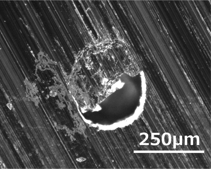
In Fig. 5 one can see the projection of the centroids of all defects in the sample on the x,y-plane of a steel sample which was milled off orthogonal to the upper side. At a range of between 50 and 75 mm from the upper side of the steel block, a huge agglomeration of mostly globular shaped defects can be found. After filtering out the artifacts, further investigation revealed that the volume of these defects follows a log-normal distribution. Figure 6(a) shows a histogram of the log-transformed volumes in log (μm³). Under the hypothesis of a log-normal distribution, log-transformed values follow a normal distribution. In the figure, the characteristic bell shape can be seen, which leads to the conclusion that the log-transformed volumes do indeed follow a normal distribution. The black curve is a fit for the theoretical normal distribution, with the distribution parameters μ = 14.687 and standard deviation σ = 1.4404 estimated via maximum likelihood from the data. To rate the quality of the fit, we plotted the empirical quantiles of the log-transformed volumes against the theoretical quantiles of the normal distribution in Fig. 6(b). Despite the deviation in the lower tail, which can be explained by the limited resolution of the camera system used for the recording, the fit seems to be a good approximation of our data. These three observations—how the defects gather in a narrow band below the surface of the upper side of the steel block, their spherical shape and the log-normal distribution of their volumes—leads to this question: What kind of defects have been detected? It is well known that nonmetallic inclusions follow the log-normal distribution18) and that they gather in a small band.10) This fact is explained by the solidification properties of steel. Solidification starts at the outer parts of the slab; thus, inclusions that have not yet been absorbed by the slag can no longer rise and are captured. They concentrate in a narrow band below the surface. The spherical shape could be an indicator of macro-oxide inclusions, which are globular in raw steel samples.9) However, further analysis of single defects in the cut images using a microscope optic (see Fig. 7) revealed that the detected defects are hollow. In the picture one can clearly see the hole in the steel surface. Using the microscope optic makes it possible to measure the depth of the hole by focusing the ground. It is approximately 20 μm deep. Another interesting detail that can be observed in the picture is that the mill presses material into the hole. Because of this, half of the hole seems to be covered by a steel cap. One possible explanation of this kind of defect is an entrapment of argon bubbles during solidification, resulting in a band similar to that of nonmetallic inclusions. Interestingly, no description of this phenomenon was found in the literature. To complete our analysis, we investigated the spatial distribution of the supposed argon bubbles. We wanted to know whether the distribution of these defects is homogeneous inside the band. To find out, we treated the centroids of the defects as a point pattern and estimated the pair correlation function g(r) from the data. The pair correlation function for the three-dimensional case is defined as
g(r)=
K'(r)
4π
r
2
for r ≥ 0, where K'(r) is the first deviation of the Ripley’s K function, which is roughly spoken the average number of points found within the distance r from a randomly chosen point (for more information see Illian et al.19)). For a point pattern with a completely spatial random distribution (CSR) g(r) is equal to one. A deviation from one can be an indication for a regularity in the pattern (g(r) ≤ 1) or a clustering of the points (g(r) ≥ 1). Figure 8 shows the pair correlation function estimated from the data using isotropic edge correction.20) Only points which centroids lie in the band between 50 mm and 75 mm on the y-axis were considered, while in the x- and z-direction no constraints were made. The first thing one can see from the plot is, that the points have a minimum inter-point distance (also called hard-core distance) of approximately 25 μm (g(r) = 0 for r ≤ 25 μm). This results from the fact, that the points in our pattern are actually spherically shaped gas bubbles, which do not overlap and which have a minimum radius of 20 μm. In the range between 25–150 μm a strong clustering is indicated by the large number of neighbors. At larger distances no correlation between the points can be seen from the graph, which could be an indication for a completely spatial distribution of the points on large scales.

Figure 9 shows a collection of defects, which are nonmetallic inclusions (verified by using a microscope) recorded in high resolution images of a steel surface 220 × 110 mm² in size. For image capture a pixel size of 2.75 μm was used. From the images one can see that, even on this scale, it is possible to identify a difference in the two-dimensional morphology of micro-inclusions. Besides the raw images of the micro-inclusions, an evidence image shows the response from the image segmentation filter. Higher values in this image correspond to a higher probability that the particular pixel belongs to the inclusion. Thus, it can be seen that automated detection of micro-inclusions on this scale is possible using our system. Using a threshold filter, the evidence image can be used to binarize the inclusions, which allows us to carry out further investigations, such as an analysis of the two-dimensional morphology.
7.3. Analysis of a Crack
Figure 10 shows the image of a crack which a human observer can clearly distinguishable from the milling grooves. However, because that the crack is very thin (at some positions just 2 to 3 pixels) it is very challenging for automatic image processing to detect this defect. Currently our image processing unit (see Section 4) is not optimized for crack detection. Using PHOT it is very likely that some parts of the crack will be detected (the structure is very irregular compared to the milling grooves), but the segmentation will result in multiple objects with some missing parts. Still, this information is enough to estimate the spatial expansion of the crack. Figure 11(a) shows the projection of the voxels belonging to the detected parts of the crack on the xy-plane. Using this technique enables the maximum width and length of the crack to be estimated. To determine the spatial expansion, we additionally projected the voxels belonging to the crack onto the xz-plane. In Fig. 11(b) one can see that the crack is present in almost every layer with a total expansion of 3.2 mm in depth.

However, at the moment we have no information about the origin of the detected cracks. They could develop during solidification, during the sample taking process or even because of the heavy mechanical stresses exerted during the milling process. Furthermore, our metrology system is not capable of applying crack opening displacement tests because we can not place stress on the steel samples and induce artificial cracks in order to measure the crack growth rate during image capture.
8. Conclusion
In this paper we have presented a new flexible detection technique for nonmetallic inclusions and other kinds of defects based on the analysis of milled steel samples. We described the camera and lighting setup and an automated positioning system, which we successfully used to record high resolution images of the steel surface. Furthermore, we addressed how we implemented image segmentation filters in order to detect the various defects and suppress periodic grooves that emerge during the milling process. A morphological analysis of the defects was carried out, which allowed us to distinguish between classes of these defects. Currently, it is possible to distinguish between globular defects, which are thought to be oxide macro-inclusions or gas bubble entrapments; cracks or parts of cracks; and artifacts from the milling process. Using a support vector machine and a manually classified test data set, an automated classification was implemented and positively evaluated. Finally, we presented the data analysis and visualization capabilities of our system and gave two concrete examples, which showed the broad range of possible analyses, that can be carried out on the data retrieved by our system.
In future, we plan to optimize every single stage of our pipeline. First of all, we want to improve the image recording step. We are currently experimenting with infrared and multispectral image recordings in order to reveal the chemical composition of nonmetallic inclusions. Combining those results with results from LIBS, we hope to find a correlation between the morphology and the chemical composition, so that our classification system can be trained with these data in order to distinguish not only among different classes of defects, but also among different kinds of non-metallic inclusions based on their chemical composition. To realize this goal, it is crucial to improve the spatial resolution of our image recording unit and enhance the image processing step so that the three-dimensional reconstruction results in a more precise reproduction of the inclusions. As a first step, it is important to provide a rating of the effective spatial resolution of our image recording system in order to make the quality comparable to system changes in the future. In this paper we quantified the quality in terms of the theoretical pixel size of the sensor. In future we want to express the quality in terms of the modulation transfer function, which can be derived from the edge response function. However, to do so, we need a standardized resolution test target with a line thickness less than 1.375 μm, which is expensive and difficult to acquire. Finally, we need to test our system with more data. At present, all volume data sets have been recorded with downsampled pixels of 20 μm in size, while our system is capable of increasing the pixel size to 2.75 μm. The next step will be to scan an entire volume of several hundred gigabytes at such a resolution to test whether our system is capable of handling such large data sets.
References
- 1) Y. Murakami: Metal Fatigue, Effects of Small Defects and Nonmetallic Inclusions, Elsevier, Oxford, (2002), 75.
- 2) E. Plöckinger and H. Straube: Die Desoxidation, Die physikalische Chemie der Eisen und Stahlerzeugung, Verlag Stahleisen, Düsseldorf, (1964), 303.
- 3) H. Jacobi and F. Rakoski: Stahl Eisen, 116 (1996), 59.
- 4) E. Steinmetz and H. U. Lindenberg: Arch. Eisenhüttenwes., 47 (1976), 199.
- 5) E. Steinmetz, H. U. Lindenberg and W. Mörsdorf: Stahl Eisen, 97 (1977), 1154.
- 6) F. Rakoski: Stahl Eisen, 114 (1994), 71.
- 7) L. Zhang and B. G. Thomas: ISIJ Int., 43 (2003), 271.
- 8) G. Vander Voort: Metallography, Principles and Practice, McGraw-Hill, New York, (1999), 472.
- 9) H. Jacobi: Stahl Eisen, 114 (1994), 45.
- 10) H. Jacobi, R. Klemp and K. Wünnenberg: Stahl Eisen, 107 (1987), 773.
- 11) H. Jacobi, H. J. Bäthmann and J. Gronsfeld: Stahl Eisen, 108 (1988), 946.
- 12) A. Fuchs, H. Jacobi, K. Wagner and K. Wünnenberg: Stahl Eisen, 113 (1993), 51.
- 13) M. Kawakami, T. Nishimura, T. Takenaka and S. Yokoyama: ISIJ Int., 39 (1999), 164.
- 14) D. Aiger and H. Talbot: Computer Vision and Pattern Recognition, IEEE, Piscataway, NJ, (2010), 295.
- 15) J. Ohser and F. Mücklich: Statistical Analysis of Microstructures in Materials Science, John Wiley, Chichester, (2000), 107.
- 16) D. Legland, K. Kieu and M. Devaux: Image Anal. Stereol., 26 (2007), 83.
- 17) K. Falconer: Fractal Geometry, Mathematical Foundations and Applications, John Wiley, Chichester, (1990), 38.
- 18) H. V. Atkinson and G. Shi: Prog. Mater. Sci., 48 (2003), 457.
- 19) J. Illian, A. Penttinen, H. Stoyan and D. Stoyan: Statistical Analysis and Modelling of Spatial Point Patterns, John Wiley, Chichester, (2008), 214.
- 20) A. J. Baddeley, R. A. Moyeed, C. V. Howard and A. Boyde: Appl. Statist., 42 (1993), 641.
- 21) L. M. Cabalin, M. P. Mateo and J. J. Laserna: Spectrochim. Acta, Part B, 59 (2004), 567.
- 22) H. M. Kuss, H. Mittelstaedt and G. Mueller: J. Anal. At. Spectrom., 20 (2005), 730.