Distribution of Particle Descending Velocity in the COREX Shaft Furnace with DEM Simulation

Abstract

Screws in COREX shaft furnace are used to discharge burdens to the latter processor - the melter gasifier. They play a very important role in the uniform drawdown pattern, which directly affects the uniform gas distribution and further the smooth operation in the COREX shaft furnace. Therefore, a three dimensional model is established based on the discrete element method (DEM) in the present work. The model is used to investigate the effect of the bottom diameter of COREX shaft furnace, the cylinder height and the screw flight diameter on particle descending velocity along the radius during discharging process. Results show that the descending velocity decreases along the radial direction. It is better to decrease the bottom diameter of COREX shaft furnace, or the screw flight diameter, or to increase the cylinder height in order to achieve a uniform descending velocity along the radius. An optimization model is also proposed for uniform drawdown pattern in the end.

1. Introduction

Screws are extensively used for transporting powders or particles in food, cement, mineral processing and agricultural industries. And they have been investigated experimentally and theoretically by many researchers. For example, Bates compared the different flow pattern by conducting a series of experiments on the combination of different screws and materials in a hopper.¹⁾ Yu and Arnold proposed a theoretical model for achieving a uniform flow pattern based on the pitch characteristic of screws.²⁾ Screws are also applied into the ironmaking field, especially the COREX process, which is composed of two reactors: the shaft furnace (hereafter “CSF”) and the melter gasifier.^3,4,5) COREX process realized its largest-scale production in terms of C-3000 in Baosteel at the end of 2007. However, due to its short history in comparison with blast furnace process, the C-3000 process faces lots of problems, such as gas distribution and burden sticking in CSF.^{6,7,8,9,10,11)} In terms of screws in CSF, eight screws are centrosymmetrically located at the bottom of CSF in order to discharge burdens into the melter gasifier for further reaction. The screws determine the particle descending velocity along the radius, which has significant effect on the gas distribution, and further on the smooth and efficient operation in CSF. However, the screws in CSF have not been investigated yet for the short history of C-3000 process. Therefore, it is necessary to systematically study the particle descending velocity along the radius in CSF during the discharging process by screws.

The discrete element method (DEM), developed by Cundall and Strack,¹²⁾ has become one of the most popular and reliable simulation methods for granular behavior. In the screw feeder or conveyor field, plenty of papers have been reported that the simulation results based on DEM coincided well with experiments and plant data.^{13,14,15,16,17,18,19,20,21,22,23)} For example, the performance of screw conveyors based on DEM was firstly conducted by Shimizu and Cundall.¹³⁾ They found that DEM is well developed and useful to analyze the performance of screw conveyors after comparing the results with previous work and empirical equations.

Therefore, in the present work, a three dimensional model of CSF is established based on DEM. The influences of the bottom diameter of CSF, the cylinder height and the screw flight diameter on the particle descending velocity are further studied by the established model. An optimal design is proposed in order to obtain a uniform drawdown in CSF at last.

2. DEM Method

In DEM, particle’s movements are described as inter-particle model, shown in Fig. 1, that a particle may collide with neighboring particles or the wall.^12,24) The model consists of spring and dashpot in the normal direction, spring, dashpot and slider in the tangential direction. Figure 2 illustrates the interactive forces between particles. At any time τ, the governing equations for particle i can be written as follows.^25,26,27)   

$$m_i\frac{d{\mathbf{V}}_i}{d\tau }=\sum _{j=1}^K({\mathbf{F}}_{cn,ij}+{\mathbf{F}}_{dn,ij}+{\mathbf{F}}_{ct,ij}+{\mathbf{F}}_{dt,ij})+m_i\mathbf{g}$$(1)

  

$$I_i\frac{d{\omega }_i}{d\tau }=\sum _{j=1}^K({\mathbf{M}}_{t,ij}+{\mathbf{M}}_{r,ij})$$(2)

Fig. 1.

Contact model in DEM.

Fig. 2.

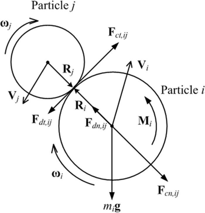
Interactive forces between particle i and j.

Where, m_i, V_i, and ω_i are the mass, translational velocity and angular velocity of particle i, respectively, and K is the number of particles in contact with particle i. I_i is the moment of inertia of particle i, given by I_i=2/5m_iR_i². The forces involved are the gravitational force, m_ig, and inter-particle forces between particle i and j, which includes the normal and tangential contact forces, F_cn,ij and F_ct,ij, and damping forces in normal and tangential directions, F_dn,ij and F_dt,ij. Torques M_t,ij and M_r,ij arise from tangential forces (F_ct,ij+F_dt,ij) and rolling friction, respectively. All the forces and torques used in the model are listed in Table 1.^28,29,30)

Table 1. Forces and torques acting on particle i.

Forces and torques	Symbols	Equations
Normal contact force	Fcn,ij	${\mathbf{F}}_{cn,ij}=–(4/3)E_{ij}{R}_{ij}{\hspace{0.17em}}^{1/2}{\delta }_n{\hspace{0.17em}}^{3/2}\mathbf{n}$
Normal damping force	Fdn,ij	${\mathbf{F}}_{dn,ij}=–2\times {(5/6)}^{1/2}\zeta {[2m_{ij}{E}_{ij}{(R_{ij}{\delta }_n)}^{1/2}]}^{1/2}{\mathbf{V}}_{n,ij}$
Tangential contact force	Fct,ij	${\mathbf{F}}_{ct,ij}=–8G_{ij}{(R_{ij}{\delta }_t)}^{1/2}\mathbf{t}$
Tangential damping force	Fdt,ij	${\mathbf{F}}_{dt,ij}=–2\times {(5/6)}^{1/2}\zeta {[8m_{ij}{G}_{ij}{(R_{ij}{\delta }_n)}^{1/2}]}^{1/2}{\mathbf{V}}_{t,ij}$
Torque by tangential forces	Mt,ij	${\mathbf{M}}_{t,ij}={\mathbf{R}}_{ij}\times ({\mathbf{F}}_{ct,ij}+{\mathbf{F}}_{dt,ij})$
Rolling friction torque	Mr,ij	${\mathbf{M}}_{r,ij}=–{\mu }_{r,ij}\left|{\mathbf{F}}_{n,ij}\right|{\omega }_{t,ij}/\left|{\omega }_{t,ij}\right|$

Where, E_ij=[(1–υ_i²)/E_i+(1–υ_j²)/E_j]^–1, R_ij=(1/R_i+1/R_j)^–1, m_ij=(1/m_i+1/m_j)^–1, G=E/(2+2υ), G_ij=[(1–υ_i)/G_i+(1–υ_j)/G_j]^–1, ς=[lne/(π²+ln²e)^1/2]^1/2, n=δ_n,ij/|δ_n,ij|, t=δ_t,ij/|δt_,ij|, V_ij=V_j–V_i+ω_j×R_j–ω_i×R_i, V_n,ij=(V_ij·n)·n, V_t,ij=(V_ij×n)×n. Note that the tangential forces (F_ct,ij+F_dt,ij) should be replaced by the maximum friction force μ_s|F_cn,ij+F_dn,ij|t when they are larger than later force.

3. Model Simulation

A COREX-3000 process was put into production at Baosteel in 2007. A three dimensional model of CSF (hereafter referred as “base model”), shown in Fig. 3, is established based on the one in Baosteel, but the size and dimensions are not the same due to the confidential agreements with Baosteel. For example, the CSF height is shortened in the model, and the CSF wall is designed vertically. However, this does not affect the laws and results on particle descending velocity. The eight screws in CSF are of same size, and the schematic diagram is presented in Fig. 4. It can be seen that the screw is with constant tooth thickness t, screw core diameter D_C and screw length L, which are 50 mm, 500 mm and 5000 mm respectively. The screw flight diameter D and pitch p are expanded along the radius and the geometric properties of screws are illustrated in Table 2.

Fig. 3.

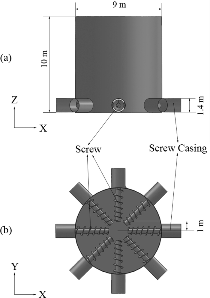
CSF model used in the simulation.

Fig. 4.

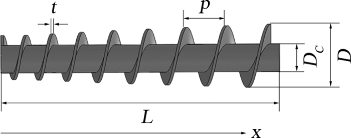
Schematic diagram of screw in CSF model.

Table 2. Geometric properties of screws in CSF model.

Number	0	1	2	3	4	5	6	7	8
D (mm)	800	800	850	900	950	1000	1050	1100	1150
p (mm)	400	450	500	550	600	650	700	750	800

Therefore, the variable screw flight diameter D(x) and pitch p(x) at any point x along the screw length can be written as   

$$D(x)=D_b+\frac{D_f–D_b}{L}x$$(3)

  

$$p(x)=p_b+\frac{p_f–p_b}{L}x$$(4)

where subscript b and f represent the beginning and finishing of screw flight diameter and pitch. Thus, the screw cross-sectional area of the screw flight A(x) can be calculated by   

$$A(x)=\frac{\pi }{4}\left[D{(x)}^2–D_C{\hspace{0.17em}}^2\right]$$(5)

Due to the work of Roberts and Willis,³¹⁾ and Yu and Arnold,²⁾ the withdrawn volume V(x) can be achieved by analytic method, which is highly recognized.   

$$V(x)={\eta }_v(x)A(x)p(x)$$(6)

where η_v is the volumetric efficiency, which is defined as the ratio of the actual volumetric flow to the maximum theoretical volumetric flow.^32,33) For a horizontal screw, η_v is defined as   

$${\eta }_v(x)=\frac{1}{tan{\alpha }_m(x)tan[{\phi }_f+{\alpha }_m(x)]+1}$$(7)

where φ_f is the angle of friction on screw flight surface. α_m(x) is the mean helix angle of the screw flight at point x along the screw length, which is given by   

$${\alpha }_m{=\text{tan}}^{-\text{1}}\left[\frac{p(x)}{\pi D_m}\right]$$(8)

where D_m is the effective mean screw diameter, which is defined as the average of the screw flight diameter and screw core diameter.

In Baosteel, CSF is charged with mixture burden of ore, pellet, coke and flux from the hopper and distributor. As the burden sizes range widely, it will take numerous time to carry out the simulation according to the actual sizes of burden. Thus the simulation select pellet as the object because the volume of pellet is larger than the others. The pellet is assumed as spherical particle in the simulation and the condition of pellet is presented in Table 3. It should be noticed that the particle diameter is enlarged. This is because it is almost impossible to do the simulation with the actual particle size in this work, for instance, the number of particles in the simulation is over 11 million if the particle diameter is five times large, and it costs over 700 hours just to generate the particles, let alone the other parts like screw rotating. Therefore, the particle diameter has to be enlarged and the accuracy of this enlargement will be discussed later.

Table 3. Pellet particle conditions in the simulation.

Parameters	Large	Medium	Small	Unit
Diameter	300	200	100	mm
Mass ratio	33.33	33.33	33.33	wt%
Number of particles	9914	34449	267711	–

The geometries in the base model, including CSF wall, screw, cylinder and so on, are made of steel, and they are called wall generally. The parameters used in the simulation are collected in Table 4.^26,27,34,35) According to Fernandez,²²⁾ the static friction coefficient between particle and screw surfaces (including the screw flight surface, the outer surface of screw shaft and so on) is set as 0.364, corresponding to the angle of friction on screw flight surface of 20°. The coefficient is smaller than that between particle and CSF wall for the consideration of that the screw may be polished by particle flow.

Table 4. Parameters used in the simulation.

Parameters	Symbols	Particle	Wall	Unit
Density	ρ	3425	7850	kg·m–3
Shear modulus	G	1×107	7.9×1010	Pa
Poisson’s ratio	υ	0.25	0.30	–
Static friction coefficient	μs	0.50	0.40	–
Rolling friction coefficient	μr	0.05	0.05	–
Restitution coefficient	e	0.60	0.50	–
Time step	τ	1×10–5		s

Where, the static friction coefficients of particle and wall stand for the coefficient of particle-particle and particle-wall, respectively, so do the rolling friction coefficient and restitution coefficient.

The simulation procedure is as follow. Firstly, build the geometry of the three dimensional model with shaft wall and screws together; Secondly, import the geometry as surface mesh into the DEM and set up all the parameters in the simulation; Thirdly, fill the CSF to 90% full with 1440 tons well-mixed pellet particles mentioned above. Then the eight screws start to rotate around their own axes in order to extrude the particles from CSF. At last, stop the simulation until the particles cannot be extruded out of the CSF any more.

In the C-3000 operation of Baosteel, it takes 6–7 hours to extrude these particles out of CSF. Thus, the screw rotating speed in the simulation has to be accelerated in order to improve the calculation time since 1 second movements of particles cost half an hour calculation time in average according to the simulation. Additionally, according to Owen and Cleary,¹⁹⁾ the particle mass flow and the average particle speed are linear functions of rotational speed of screw from 200 RPM to 1400 RPM for horizontal screw conveyor. Similar results about mass flow are also found in Shimizu and Cundall,¹³⁾ Moysey and Thompson^15,16) ’s work.

Three levels with 1 m height are examined in order to analysis the particle descending velocities along the radius. The schematic diagram is shown in Fig. 5.

Fig. 5.

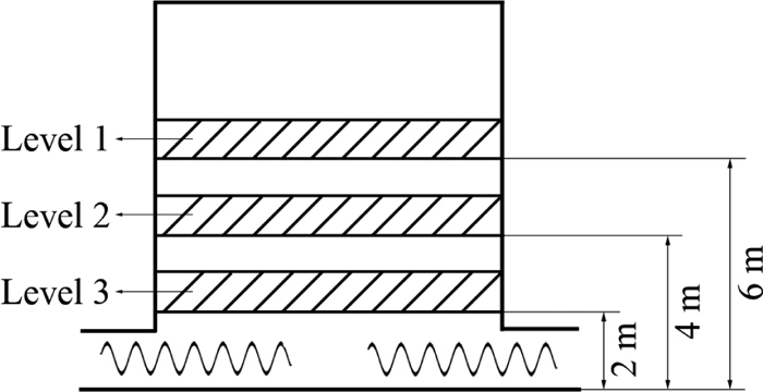
Schematic diagram of different levels.

A series of same sized cuboids with 1 m height are selected in the three levels to measure the particle velocities along radius around peripheral directions. And the peripheral locations are defined in Fig. 6, corresponding to the top view of CSF in Fig. 3. In Fig. 6, the plus X and Y directions are defined as 0° and 90°. It can be seen that there are screws in the directions of 0°, 45°, 90°, 135°, 180°, 225°, 270° and 315° (hereafter “screws”) while there are no screws in the directions of 22.5°, 67.5°, 112.5°, 157.5°, 202.5°, 247.5°, 292.5° and 337.5° (hereafter “no screws”). The X-direction and Y-direction component velocities of particle are too small to be considered after confirmation. Therefore, the paper only investigates the Z-direction component velocity of particle. The Z-direction velocity varies at first and then becomes relatively stable during the screw extruding process, thus the velocities in the relatively stable period are averaged to represent the velocity at the point of radius.

Fig. 6.

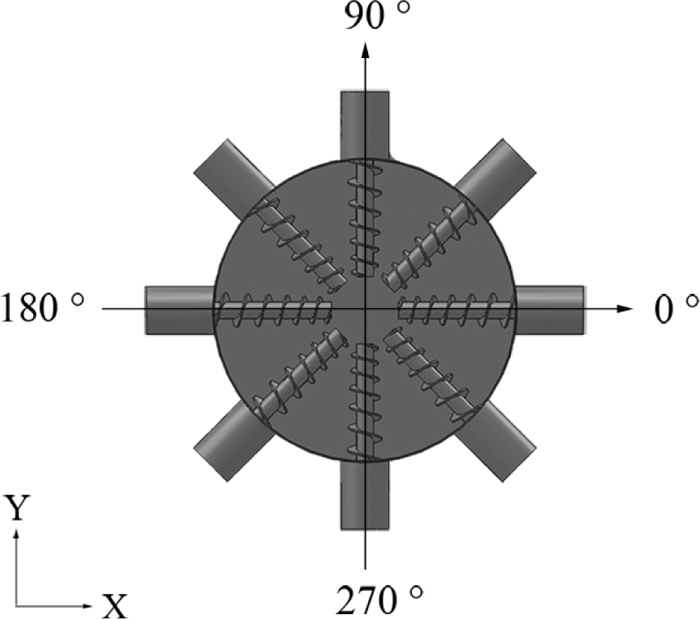
Schematic diagram of peripheral locations.

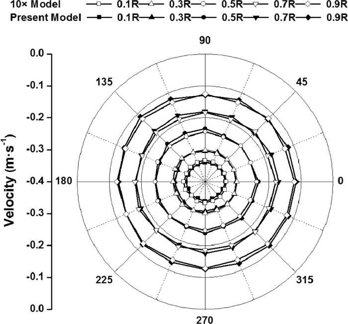
In order to validate the accuracy of the assumption of particle diameter, a model is also established basing on 10 times large particle diameters (hereafter “10× model”), and the diameters of particles are 60 mm, 120 mm and 180 mm. The numbers of large, medium and small are 45865, 154568 and 1236125, respectively. And this simulation cost about 360 hours to complete. Figures 7, 8 and 9 show the comparisons of the Z-direction velocities along peripheral directions for the 10× model and the base model in Level 1, 2 and 3, respectively , where the negative velocities suggest particle descending velocity is opposite to the positive Z direction.

Fig. 7.

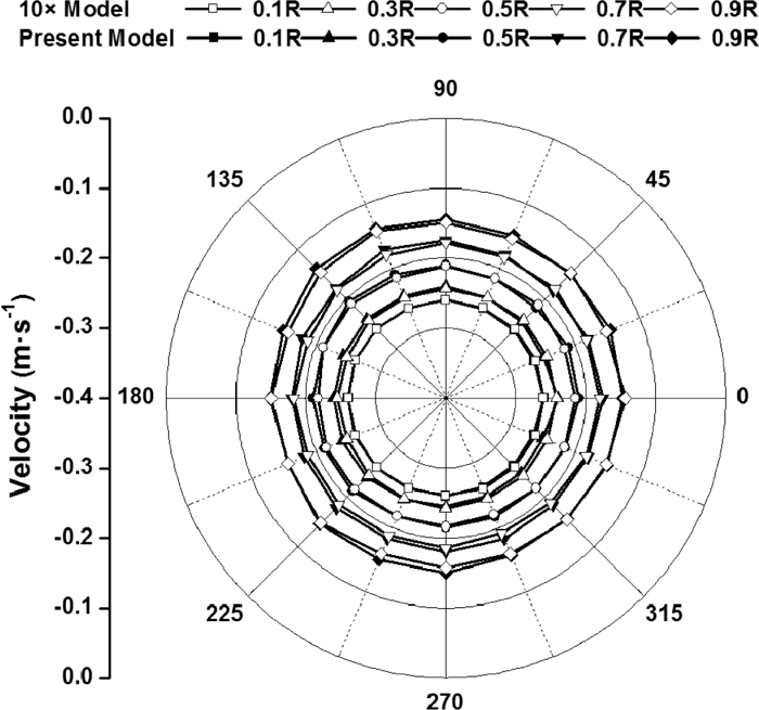
Comparison of Z direction velocity between two models in Level 1.

Fig. 8.

Comparison of Z direction velocity between two models in Level 2.

Fig. 9.

Comparison of Z direction velocity between two models in Level 3.

It can be seen that the Z direction velocities for the two models in the three levels show slight differences. Additionally, it should be noticed that the particle diameter in the present model is close to the radius of the screw shaft. The ratio of the screw diameter to the average particle diameter is 2.5 in the present model, and it is about 4.17 in the 10× model. In the work of Fernandez et al.,²²⁾ the screw shaft diameter is from 22.5 mm to 37.5 or 45 mm, and the diameter of the spherical particle is 5 mm, which leads to a the ratio of 4.5 to 9. And in the work of Hu et al.,²⁰⁾ the ratio is about 3.93. Thus, the ratio of 10× model is reasonable according to these research. Since there is almost no difference between the present model and 10× model, the assumption of enlarging particle diameter to 200 diameter has no influence on the particle movement in the CSF. Therefore, the present model is reasonable and can used to investigate the particle movement in CSF.

Since the screws are periodically installed in the bottom, it is thought that the un-uniform movements of particles along the peripheral directions appear in the lower part. Therefore, the cross-sections, parallel to the X-Y plane, of Z direction descending velocity of particles are extracted 0.75 m and 2.5 m high from the CSF bottom and shown in Fig. 10.

Fig. 10.

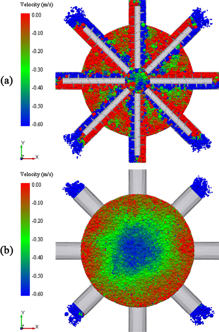
Cross-sections (perpendicular to the Z axis) of velocity distribution (a) 0.75 m and (b) 2.5 m high from the CSF bottom. (Online version in color.)

It can be seen that the particle descending velocity between screws is much smaller than that above screws. This is because the particles between screws cannot be affected by the screws directly. It should be noticed that the velocities along peripheral directions in Fig. 10(b) seem to be uniform. In order to evaluate them quantificationally, the descending velocities are extracted in level 3 and presented in Fig. 11.

Fig. 11.

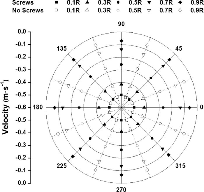
Comparison of velocities along the radius between screws and no screws areas.

The velocities show slight differences in both screws and no screws areas. This means the velocities are almost uniform in peripheral directions in level 3, so are in level 1 and 2. Therefore, the cross-section of particle descending velocity along 180°–0° direction is used to represent the velocity distribution in the CSF visually, which is shown in Fig. 12, where the red particle means small descending velocity while the blue one means large velocity.

Fig. 12.

Cross-section of particle descending velocity along 180°–0° direction in base model. (Online version in color.)

There exists a blue part in the central area of CSF, which means that the particle descending velocity in the central area is the largest. The reason is that the effect of the first flight is quite large and direct for the particle movement, which is also found in Yu and Arnold’s work.²⁾ The velocity reduces with the increase of the height from the CSF bottom and from center to wall areas. In order to study the velocity quantificationally, the average of velocities in the above 16 directions is calculated and used to represent the velocity along radial direction, which is illustrated in Fig. 13.

Fig. 13.

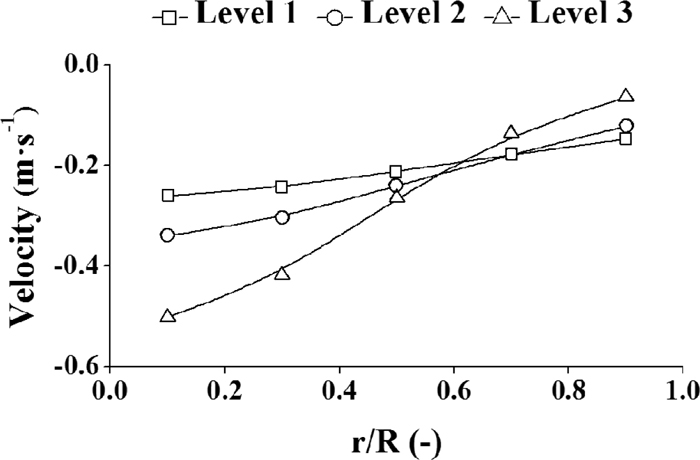
Z-direction velocities along the radius in base model.

It can be seen from Fig. 13 that the descending velocities in each level decrease along radial direction. And the difference between the maximum and minimum velocities is the biggest at Level 3, 0.438 m·s^–1, while it is smallest at Level 1, 0.113 m·s^–1, which implies that the velocity along the radius is relatively even at higher level of CSF while it becomes uneven at lower level of CSF. Specifically, the standard deviations from Level 1 to Level 3 are 0.041, 0.080 and 0.165, respectively. Thus, it is of necessity to investigate the velocities along the radius at different conditions in order to obtain a uniform velocity distribution since the uniform drawdown pattern is the best way to discharge materials from CSF.

4. Results and Discussion

The factors investigated in this paper include the bottom diameter of CSF, cylinder height and screw design.

4.1. The Bottom Diameter of CSF

In this paper, the bottom diameter of CSF refers to the diameter at the top plane of screws. Figure 14 illustrates the schematic diagram of different bottom diameters of CSF.

Fig. 14.

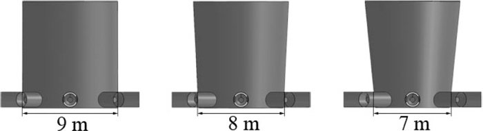
Schematic diagram of different bottom diameters of CSF.

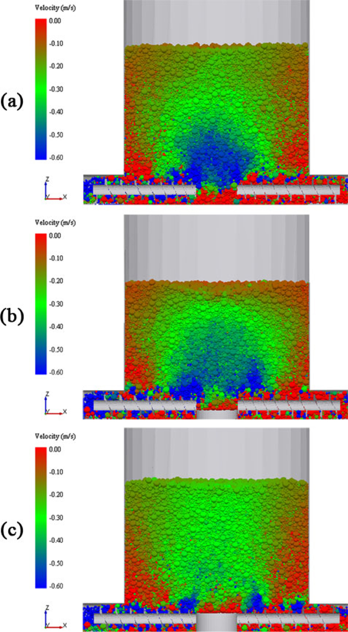
It can be seen that the CSF becomes narrower with the bottom diameter of CSF decreasing. The visual representation of velocity distribution is shown in Fig. 15.

Fig. 15.

Cross-sections of velocity distribution at different bottom diameters of CSF (a) 9 m, (b) 8 m and (c) 7 m. (Online version in color.)

In Fig. 15, the low velocity areas at the both sides of CSF bottom turn to smaller with the bottom diameter of CSF decreasing while other areas almost remain unchanged. Therefore, the velocities along the radius in three levels are extracted and presented in Fig. 16 in order to study the phenomenon quantificationally.

Fig. 16.

Velocities along the radius at different bottom diameters of CSF.

In three levels, the descending velocities within 0.4R are almost the same at different bottom diameters of CSF, while they increase a little with the bottom diameter of CSF decreasing. For example, in the case of 7 m bottom diameter, the descending velocities at 0.9R from Level 1 to Level 3 increase by 16.85%, 36.99% and 111.10% respectively comparing with the base model. This is because the length of the screw below the CSF becomes shorter, which leads to the burden volume above screw relatively increase, and further increases the volumetric efficiency.

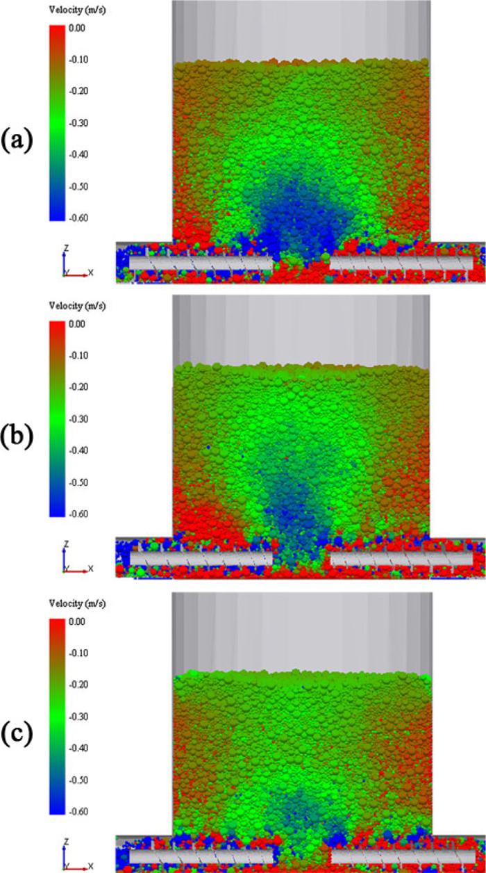
4.2. The Cylinder Height

Since the descending velocity in central area is largest in each level of base model, a cylinder with 2 m diameter is placed on the bottom of CSF in order to limit the velocity in central area. The cylinder heights investigated are 0 m, 0.5 m and 1 m respectively, and the cylinder with 0 m height refers to the base model. Figure 17 illustrates the cross-sections of velocity distribution at different cylinder heights.

Fig. 17.

Cross-sections of velocity distribution at different cylinder heights (a) 0 m, (b) 0.5 m and (c) 1 m. (Online version in color.)

It can be seen that the blue area of high descending velocity is becoming smaller with the increase of cylinder height. This means that the descending velocity in the central area is limited by the cylinder. The velocities along the radius are shown and analyzed in Fig. 18.

Fig. 18.

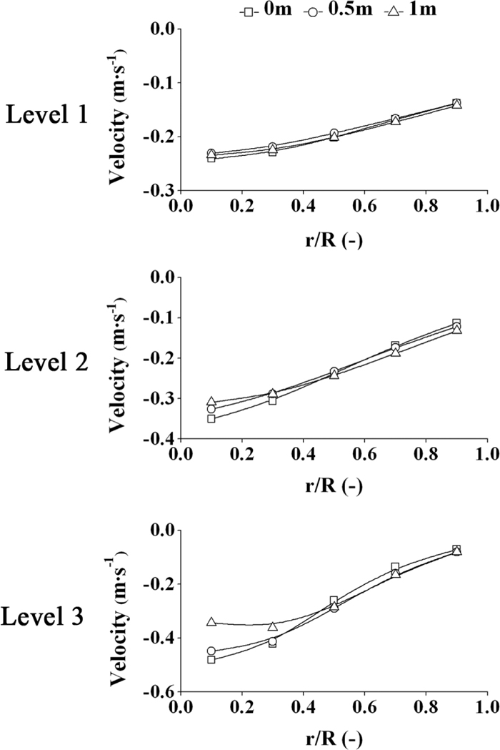
Velocities along the radius at different cylinder heights.

In Level 1, there is almost no difference for velocities among the three cylinder heights. In Level 2, the descending velocities beyond 0.3R are almost the same while they become smaller with the increase of cylinder heights within 0.3R. Specifically, the descending velocity in the case of 1 m cylinder height decreases by 11.76% compared with that of base model. In Level 3, the descending velocities also decrease before 0.5R with the cylinder heights rising, and the velocity in the case of 1 m cylinder height is 28.54% smaller than that of base model. And the standard deviation in Level 3 decreases from 0.158 to 0.108. This implies that the descending velocities in the central part reduce when the cylinder height increases, especially in level 2 and 3, which help to obtain the evenness of drawdown patterns.

As for the C-3000 in Baosteel, there is a man-made deadman at the central bottom of CSF. The diameter of the deadman is the same as the empty area formed by the eight screws and the height of the deadman’s cylinder part is 0.9 m, close to the height in this work, which validates the results of this paper.

4.3. The Screw Flight Diameter

The screw flight diameter D used in the base model is from 800 mm to 1150 mm. It can be inferred that the screw flight diameter near to the center is a little large since the descending velocity in the center is higher. Thus, the screw flight diameter near the center is reduced to decrease the descending velocity in central area. The condition of different screw flight diameter is tabulated in Table 5, where the pitch p, screw core diameter D_C and the end of screw flight diameter D are the same as base model.

Table 5. Geometric properties of different screw flight diameters.

Number		0	1	2	3	4	5	6	7	8
D (mm)	Screw A	725.0	725.0	785.7	846.4	907.1	967.8	1028.5	1089.2	1150.0
	Screw B	650.0	650.0	721.5	793.0	864.5	936.0	1007.5	1079.0	1150.0

According to Yu and Arnold’s work,²⁾ the screw can achieve a uniform drawdown pattern if the profile coefficients f_p of all pitches are equal to 1. Specifically, f_p=1 means a uniform withdrawal performance while f_p=0 means no increment in a pitch. The profile coefficient f_p of kth pitch is defined as   

$$f_{pk}=\frac{A_{ak}-A_{ak-1}(p_{k-1}/p_k)}{A_{a1}}$$(9)

where A_ak is the average effective area at pitch k, which can be calculated by   

$$A_{ak}=\frac{\underset{x_{k-1}}{\overset{x_k}{\int }}{A}_k(x){\eta }_v(x)dx}{x_k-x_{k-1}}$$(10)

Therefore, the profile coefficients f_p from No.2 to No. 6 pitch (only six pitches are working in the CSF, the other two pitches are in the casing.) for Base model, Screw A and Screw B are calculated and presented in Fig. 19.

Fig. 19.

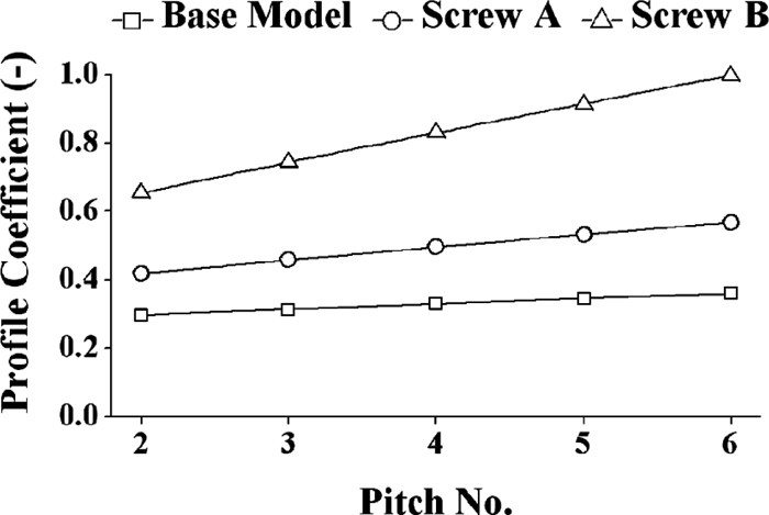
Profile coefficients at different screw flight diameters.

It can be seen from Fig. 19 that the f_p increases from No. 2 to No.6 pitch for all three screws, and the f_p slope for Screw B is largest, the next is Screw A, the screw of Base model is the smallest. And the law is the same as Yu and Arnold’s for the case of variation of the screw flight diameter. It should be noticed that the f_p of No. 6 pitch for Screw B is close to 1. This means that the design of screw flight diameter is reasonable and measures for uniform drawdown pattern should be focused on other pitches.

The geometry is rebuilt by replacing all the screws in the base model with screw A or B, and then the geometry is imported as surface mesh into the DEM. Finally carry out new simulations from the initial beginning by setting all the parameters. The results of velocity distribution are presented in Figs. 20 and 21.

Fig. 20.

Cross-sections of velocity distribution at different screw flight diameters (a) Base Model, (b) Screw A and (c) Screw B. (Online version in color.)

Fig. 21.

Velocities along the radius at different screw flight diameters.

In Fig. 20, it can be seen that the high descending velocity of blue area is shrinking with the decrease of screw flight diameter. This can be also found in Level 1 of Fig. 21, the descending velocities for Screw B are smaller than those for base model and Screw A, and they are more stable. In Level 2, there exists a turning point-0.6R; the descending velocities are smallest for Screw B and biggest for the base model before the turning point, while the biggest and smallest velocities reverse after the turning point. Thus the velocity at 0.1R in the case of Screw B decrease by 18.48% comparing with that of the base model and the standard deviation decreases from 0.087 to 0.055. This is because the screw design for Screw A and B weaken the entrainment capability of inner part of screw. In Level 3, the turning point changes to be 0.5R, and the range for velocities decrease is becoming large. The velocity at 0.1R and the standard deviation in the case of Screw B decrease by 21.37% and 32.91%. It can be conclude that the velocity distribution along the radius turns to be stable when the screw flight diameter reduces.

4.4. The Optimization Model

According to previous simulations, the bottom diameter of CSF and the screw flight diameter should be reduced while the cylinder height should be increased in order to achieve an evener velocity along the radius. Thus, an optimization model is established by combining the above factors. The bottom diameter of optimization model is 7 m since the angle between the shaft wall and the vertical line has reached over 6°, which is the limit of CSF angle. The cylinder height is 1 m for the cylinder top has reached the top of screw shaft, and the uniform drawdown will be worsen if the height increases. Screw B is also used in the model because profile coefficients f_p of No. 6 flight is near 1, which means a uniform drawdown pattern. Because the factors except screw flight diameter investigated in our work is quite new in this field, there is no calculation model available for the optimized model combining all the factors. Additionally, the mathematical model is also our work in the near future, and we hope to work it out and report it soon. The cross-section of velocity distribution in the optimization model is presented in Fig. 22.

Fig. 22.

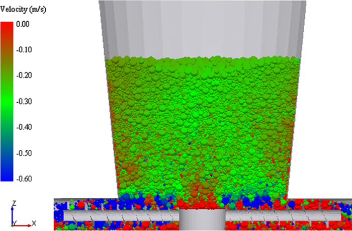
Cross-section of velocity distribution in optimization model. (Online version in color.)

It can be found that the velocity distribution is almost uniform except few red area of low descending velocity. Then the velocities along the radius between the base model and the optimization model are compared in Fig. 23.

Fig. 23.

Velocities along the radius between base model and optimization model.

In Fig. 23, the descending velocities along the radius for the optimization model seem flatter than those of the base model in each level. And the range of velocity values becomes narrower for the three levels, quite different from that of the base model. Specifically, the standard deviations from Level 1 to Level 3 decrease from 0.038, 0.087 and 0.158 to 0.024, 0.031 and 0.034, respectively. And the difference between largest and smallest descending velocities decreases from 0.410 m·s^–1 to 0.086 m·s^–1. Therefore, the velocity distribution of the optimization model is more reasonable for discharging materials evenly. Thus the paper has proposed a practical way to improve the descending velocity along the radius by optimizing some parameters. Since Baosteel decided to move the COREX process from Shanghai to Xinjiang, the results in this paper can help to optimize the design of CSF greatly.

5. Conclusions

The paper establishes a three dimensional model of CSF to study the particle descending velocity along the radius based on DEM. The factors investigated include the bottom diameter of CSF, the cylinder height and the screw flight diameter. In the base model, the descending velocities decrease along the radial direction, and the unevenness of the velocities for the lower part of CSF is the greatest throughout the CSF. To reduce the bottom diameter of CSF increases the descending velocities beyond 0.4R, while to increase the cylinder height or to decrease the screw flight diameter help to restrain the descending velocities in the central area of CSF. Therefore, an optimization model is proposed in order to achieve a uniform descending velocity along the radius of CSF, thus having a better gas distribution and further efficient operation. The optimization model has improved the evenness of descending velocity along the radius greatly, which provides a numerical basis and technical direction for COREX to improve and design CSF.

Further simulation will be carried out to investigate the effect of irregular particle shapes. This will also take into account the effect of gas flow, particle softening and shrinkage, and multiphase flow inside the entire CSF. Work on these aspects is in progress and will be reported hopefully in the near future.

Acknowledgement

The authors would like to thank Mr. Jian Xu from Chongqing University for suggestions on this work and Miss Daichun Wei for language review.

Nomenclature

A cross-sectional area of screw flight (m²)

A_ak the average effective area (m²)

D screw flight diameter (m)

D_C screw core diameter (m)

D_m the effective mean screw diameter (m)

e restitution coefficient (–)

E Young’s modulus (Pa)

f_p profile coefficient (–)

F force between particles (N)

g gravitational acceleration (m·s^–2)

G shear modulus (Pa)

I moment of inertia (kg·m^–2)

K particle number in contact with particle i

L screw length (m)

m mass of particle (kg)

M torque on particle (N·m)

n unit vector in normal direction

p screw pitch (m)

R particle radius (m)

x point along screw length (m)

t tooth thickness (m)

t unit vector in tangential direction

V velocity (m·s^–1)

V withdraw volume (m³)

Greek letters

α_m mean helix angle of the screw flight (°)

δ displacement (m)

ζ damping ratio (–)

η_v volumetric efficiency (–)

φ_f angle of friction on screw flight surface (°)

μ friction coefficient (–)

ρ density (kg·m^–3)

τ time (s)

υ Poisson’s ratio (–)

ω angular velocity (rad·s^–1)

Subscripts

b beginning point

c contact

d damping

f finishing point

i ith particle

ij between particle i and j

j jth particle

n normal component

r rolling

s static

t tangential component

Abbreviations

DEM discrete element method

CSF COREX shaft furnace

RPM revolutions per minute

References

• 1)   L.  Bates: J. Manuf. Sci. Eng., 91 (1969), 295.
• 2)   Y.  Yu and  P. C.  Arnold: Powder Technol., 88 (1996), 81.
• 3)   E.  Ottenschlaeger,  W.  Kepplinger,  G.  Papst and  R.  Hauk: MPT, 9 (1986), 24.
• 4)  Anon: Steel Times Int., 13 (1989), 24.
• 5)   A.  Eberle,  E.  Eichberger,  C.  Bohm,  G.  Leonard and  H.  Wetzling: Iron Steel Eng., 75 (1998), 25.
• 6)   A.  Eberle,  D.  Siuka and  C.  Böhm: Stahl Eisen, 126 (2006), 31.
• 7)   W. G.  Li: 3rd Baosteel Biennial Acad. Conf., SSTLPH, Shanghai, (2008), A75.
• 8)   Q.  Zhang and  L.  Guo: 3rd Baosteel Biennial Acad. Conf., SSTLPH, Shanghai, (2008), A219.
• 9)   S.  Wu,  J.  Xu,  S.  Yang,  Q.  Zhou and  L.  Zhang: ISIJ Int., 50 (2010), 1032.
• 10)   J.  Xu,  S.  Wu,  M.  Kou and  K.  Du: ISIJ Int., 53 (2013), 576.
• 11)   S.  Wu,  J.  Xu,  J.  Yagi,  X.  Guo and  L.  Zhang: ISIJ Int., 51 (2011), 1344.
• 12)   P. A.  Cundall and  O. D. L.  Strack: Geotechnique, 29 (1979), 47.
• 13)   Y.  Shimizu and  P. A.  Cundall: J. Eng. Mech., 127 (2001), 864.
• 14)   P. W.  Cleary: Eng. Computation., 21 (2004), 169.
• 15)   P. A.  Moysey and  M. R.  Thompson: Polym. Eng. Sci., 44 (2004), 2203.
• 16)   P. A.  Moysey and  M. R.  Thompson: Powder Technol., 153 (2005), 95.
• 17)   H.  Hong,  J. A.  Covas and  A.  Gaspar-Cunha: AIP Conf. Proc., American Institute of Physics, Porto, 908 (2007), 1537.
• 18)   P. W.  Cleary: Eng. Computation., 26 (2009), 698.
• 19)   P. J.  Owen and  P. W.  Cleary: Powder Technol., 193 (2009), 274.
• 20)   G.  Hu,  J.  Chen,  B.  Jian,  H.  Wan and  L.  Liu: Int. Conf. Mech. Autom. Control Eng., MACE, IEEE Computer Society, Washington, DC, USA, (2010), 927.
• 21)   P. J.  Owen and  P. W.  Cleary: Prog. Comput. Fluid Dy., 10 (2010), 327.
• 22)   J. W.  Fernandez,  P. W.  Cleary and  W.  McBride: Chem. Eng. Sci., 66 (2011), 5585.
• 23)   M.  Kimata,  Y.  Endo,  K.  Banzai and  M.  Hasegawa: Chem. Eng. Tran., 25 (2011), 785.
• 24)   J.  Zhang,  Z.  Hu,  W.  Ge,  Y.  Zhang,  T.  Li and  J.  Li: Ind. Eng. Chem. Res., 43 (2004), 5521.
• 25)   Y.  Yu and  H.  Saxén: Chem. Eng. Sci., 65 (2010), 5237.
• 26)   Y.  Yu and  H.  Saxén: ISIJ Int., 52 (2012), 788.
• 27)   Z. Y.  Zhou,  H. P.  Zhu,  A. B.  Yu,  B.  Wright and  P.  Zulli: Comput. Chem. Eng., 32 (2008), 1760.
• 28)   A.  Di Renzo and  F. P.  Di Maio: Chem. Eng. Sci., 59 (2004), 525.
• 29)   Y. C.  Zhou,  B. D.  Wright,  R. Y.  Yang,  B. H.  Xu and  A. B.  Yu: Physica A, 269 (1999), 536.
• 30)   Y.  Tsuji,  T.  Tanaka and  T.  Ishida: Powder Technol., 71 (1992), 239.
• 31)   A. W.  Roberts and  A. H.  Willis: P. I. Mech. Eng., 176 (1962), 165.
• 32)   A. W.  Roberts,  K. S.  Manjunath and  W.  McBride: 4th Int. Conf. on Bulk Mater., Storage, Handling and Trans., 7th Int. Symp. on Freight Pipelines, Institution of Engineers, Australia, (1992), 333.
• 33)   A. W.  Roberts and  K. S.  Manjunath: Pro. Tech. Prog. Powder and Bulk Solids Conf. and Exbit., Reed Exhibition Companies, USA, (1994), 189.
• 34)   H.  Mio,  S.  Komatsuki,  M.  Akashi,  A.  Shimosaka,  Y.  Shirakawa,  J.  Hidaka,  M.  Kadowaki,  S.  Matsuzaki and  K.  Kunitomo: ISIJ Int., 49 (2009), 479.
• 35)   G.  Hu: Analysis and Simulation of Granular System by Discrete Element Method Using EDEM, Wuhan University of Technology Press, Wuhan, (2010).