Active Vibration and Flatness Control of a Strip in a Continuous Galvanizing Line using Positive Position Feedback Control

Abstract

In this paper, we propose active vibration control of a strip in a continuous galvanizing line (CGL) using positive position feedback (PPF) control. The control system includes five pairs of electromagnetic actuators and controllers. First, the overall system was modeled using the three-dimensional finite element modeling (FEM) package ANSYS. The Krylov subspace technique was then used to reduce the order of the model. Finally, PPF control was applied to control the vibration. The stability condition was derived from the stiffness matrix concept, which shows the relationship between the DC gain of the controller and that of the system. Root locus analysis was performed to validate the stability condition derived. The results of the software simulations and the experiments demonstrate the effectiveness of the proposed controller under various tension conditions.

1. Introduction

The primary function of a continuous galvanizing line (CGL) is to coat a steel strip in a thin layer of zinc, enhancing the corrosion resistance of the final product. After the strip is cleaned, annealed, and cooled down to the temperature of molten zinc, the strip enters the zinc pot and travels around three rollers, which redirect it up through an air knife system (Fig. 1). The air knives blow off the excess molten zinc and control the coating thickness.

Fig. 1.

Typical CGL process layout with electromagnet vibration control system.

During the processing, the strip develops longitudinal and transverse curvatures due to the bending action of the sink roller under tension.¹⁾ Moreover, vibration may be invoked by many sources such as the eccentricity of the rotating rollers, air pressure differences between the air knives, and tension fluctuations due to speed mismatch between the rollers. Accordingly, the curvature and the vibration of the strip cause uneven coating on the strip and result in a poor-quality strip. To eliminate these, three kinds of vibration-absorbing schemes are currently used. One of these involves adjusting the tension and line speed.²⁾ However, increasing the tension causes the sink roller’s bush and sleeve to wear out quickly. Another approach is to introduce passive damping by squeezing the strip with rollers.³⁾ Although this absorbing scheme is effective, a disadvantage of this method is that it may cause surface defects such as scratches if the surface of the roller is contaminated. The final approach relies on noncontact active vibration control using electromagnetic actuators.^4,5,6)

The difficulties in active vibration control of the strip arise from the fact that the strip must be considered as a multimodal system with many frequency modes.⁷⁾ It is very hard to describe the motion of the strip in a simple model because it moves in a three-dimensional space. Modeling the strip accurately yields a very high-order model.^8,9) Only a noncontacting position feedback sensor can be used because the strip is moving in a real situation. For these reasons, state feedback control cannot be used to control the vibration of the strip because it may give rise to the well-known phenomenon of spill-over.¹⁰⁾ Inoue et al.⁵⁾ studied spill-over of a strip where the axial direction movement was modeled by a finite element method. However, they did not consider the lateral movement of the strip. They used a proportional integral (PI) controller with a phase-lead compensator for electromagnet control. O. Bruls et al.⁶⁾ used a model that neglected the global motion of the strip and the Craig-Bampton substructuring technique in model reduction. Although they employed proportional and derivative (PD) feedback control in the simulation, they did not consider spill-over.

In this paper, we propose active control of the flatness of the strip using positive position feedback (PPF) control. The control system consists of five pairs of electromagnetic actuators. First, the overall system was modeled using state equations of the motion of the strip based on three-dimensional finite element modeling (FEM) with ANSYS. Next, the Krylov subspace technique was used to reduce the order of the state equations. Finally, decentralized PPF control was applied for vibration control, with each actuator operated by feeding back the corresponding magnitude of vibration at the same location. The stability condition for the control system was derived from the stiffness matrix concept. The derived stability condition shows the relationship between the DC gain of the controller and that of the system. The gain of the controller was adjusted according to the stability condition under various tension values because the DC gain of the system changes with the tension. Root locus analysis of the closed-loop control system was performed to validate the derived stability condition. A computer simulation was performed for various filter frequencies and tension values. The experimental results demonstrate the effectiveness of the controller under various tension conditions.

This paper is organized as follows. In Section 2, FEM of the strip and model order reduction using the Krylov subspace technique are formulated. Section 3 presents the stability condition and the design of the controller. In Section 4, computer simulations performed to validate the stability condition are presented. In Section 5, hardware experimental results are provided, and the conclusion is given in Section 6.

2. Finite Element Model of the Strip

This section outlines the mathematical modeling of the strip under tension. The commercial finite element package ANSYS was used for three-dimensional full-scale system analysis and system matrix extraction. FEM leads to a high-order full-scale system model. The corresponding reduced-order small-scale model was then derived based on second-order Krylov subspace methods. The rectangular strip 1200-mm wide and 2000-mm high was investigated. The actual strip was placed in the experimental set-up, as shown in Fig. 2.

Fig. 2.

Pilot test equipment for active vibration control.

2.1. Three-dimensional Mathematical Modeling

All elements are represented with a quadrilateral shell element in three dimensions, which has both bending and membrane properties associated with displacements and rotations. The element has 24 independent degrees of freedom consisting of q_k = [ u_x,k, v_y,k, w_z,k, θ_x,k, θ_y,k, θ_z,k ] at each of its four nodes, as shown in Fig. 3. The vector q_k is used to denote the generalized nodal displacement vector, and subscripts x, y, z, and k denote the directions and node number. The total degree of freedom of the system denoted N are determined by the total degree of freedom of the elements and that of the boundary conditions. The number of nodes and elements used in the finite element model are summarized in Table 1. The size of the system matrix is the same as the total degree of freedom of the system. We call this system a full-scale system. The generalized nodal force input vector for corresponding q_k is defined by F_k = [ f_x,k, f_y,k, f_z,k, m_xx,k, m_yy,k, m_zz,k ] , the elements of which are nodal forces and moments in the x, y, z direction. By combining all the elements, the finite element model of the strip leads to full-scale dynamic equations of motion in the following form:   

$$\mathbf{M}\ddot{\mathbf{q}}(t)+\mathbf{D}\dot{\mathbf{q}}(t)+\mathbf{K}\mathbf{q}(t)=\mathbf{F}(t)$$(1)

where $\mathbf{M},\mathbf{D},\mathbf{K}\in {ℝ}^{N\times N}$ , $\mathbf{q}(t)={[{\mathbf{q}}_1,{\mathbf{q}}_2,\cdots {\mathbf{q}}_k,\cdots ]}^T\in {ℝ}^{N\times 1}$ , and $\mathbf{F}(t)={[{\mathbf{F}}_1,{\mathbf{F}}_2,\cdots ,{\mathbf{F}}_k,\cdots ]}^T\in {ℝ}^{N\times 1}$ are the mass, damping, stiffness matrix, generalized displacement vector, and generalized force input vector of the full-scale system.

Fig. 3.

Shell element.

Table 1.Information on the finite element model.

Params	Value [unit]
Element type	Shell63
Number of node	651
Number of element	600
Number of total DOF	3654
Thickness of strip	0.8 [mm]
Width of strip	1200 [mm]
Length of strip	2000 [mm]
Young’s modulus	200e9 [N/m2]
Poison ratio	0.3
Specific weight	7850 [kg/m3]

2.2. Modal Analysis

Modal analysis of the system in Eq. (1) without damping (i.e. D = 0) provides information on dynamic characteristics of the strip such as its natural frequency and mode shape. Figures 4(a), 4(b), and 4(c) show the finite element model, displacement, and stress distribution from prestress analysis. Uniform stress was distributed throughout whole strip owing to its simple rectangular shape. The results of the prestress analysis against tension were updated in FE model for modal analysis. Tension produced a stiffening effect and considerably increased the natural frequencies. Figure 5 shows the first six mode shapes of the tensioned strip. Generally, the vibratory mode (n_x, m_y) of a plate is distinguished by the number of nodal lines in the horizontal (n_x) and vertical direction (m_y), as shown in Fig. 5. Note that nodal lines are lines at which two standing waves add with opposite phase and cancel each other out, so any actuator or sensor located at these lines does not contribute to vibration control for the mode (n_x, m_y). For instance, vertical modes such as mode (0,1), mode (1,1) and mode (2,1) can not be controlled by actuators arranged as in Fig. 2 because all of them are located on vertical modal line m_y = 1. But horizontal vibrations, especially major mode (0,0) and transverse curvature of strip can be controlled. Vibratory mode and their natural frequencies are listed in Table 2.

Fig. 4.

Finite element model.

Fig. 5.

Vibratory mode shapes.

Table 2.Natural frequencies of the pretensioned strip.

No	Mode shape		Natural frequency[Hz]
	nx	my	600 [kgf]	800 [kgf]	1300 [kgf]
1	0	0	7.3222	8.3986	10.6092
2	1	0	9.8396	11.2858	14.2613
3	0	1	15.5593	17.7258	22.2082
4	2	0	22.3739	25.5476	32.1018
5	1	1	23.1711	26.0802	32.1543
6	2	1	23.5251	26.8180	33.6325
7	3	1	26.9873	30.5867	38.0833
8	0	2	32.7144	36.3892	43.7847
9	1	2	37.0351	37.0596	45.2237
10	3	1	39.5129	44.4646	55.1420

2.3. Full-scale State Space Representation

Among many nodes, five points in Fig. 2 are assumed to be excited by magnetic actuators in the z-direction. The forces excited by the electromagnet are defined by f_z,EMi (i=1~5), where subscript i indicates the number of the magnetic actuator. The displacements measured by collocated sensors are defined by w_z,j (j=1~5), where subscript j denotes the number of the sensor. Then, the system input, output vector can be represented as $\mathbf{u}={[u_1,u_2,u_3,u_4,u_5]}^T\in {ℝ}^{5\times 1}$ and $\mathbf{y}={[y_1,y_2,y_3,y_4,y_5]}^T\in {ℝ}^{5\times 1}$ , respectively, where u_i = f_x,EMi and y_j = w_z,j. The input matrix $\mathbf{B}\in {ℝ}^{N\times 5}$ and the output matrix $\mathbf{C}\in {ℝ}^{5\times N}$ can be defined for the corresponding input and output vectors. Consequently, the dynamic model can be represented as:   

$$\{\begin{array}{l}\mathbf{M}\ddot{\mathbf{x}}(t)+\mathbf{D}\dot{\mathbf{x}}(t)+\mathbf{K}\mathbf{x}(t)=\mathbf{B}\mathbf{u}(t)\\ \mathbf{y}(t)=\mathbf{C}\mathbf{x}(t)\end{array}$$(2)

Since FEM model in Eq. (2) is linear, the superposition principle can be used. For the j-th input u_j and the i-th output y_i , by introducing intermediate state vector x_j , dynamic model in Eq. (2) can be rewritten as the linear combination form:   

$$\{\begin{array}{l}\mathbf{M}{\ddot{\mathbf{x}}}_j(t)+\mathbf{D}{\dot{\mathbf{x}}}_j(t)+\mathbf{K}{\mathbf{x}}_j(t)={\mathbf{B}}_j{u}_j(t)\\ y_i(t)={\mathbf{C}}_i\cdot \sum _{j=1}^5{\mathbf{x}}_j(t)\end{array},\hspace{1em}i=1~5,j=1~5$$(3)

where, B_j and C_i are j-th column vector of input matrix B and i-th row vector of output matrix C. To find the individual relationship between the j-th input and i-th output, intermediate output variable y_ij was introduced into the linear combination output y_i(t) in Eq. (3) as   

$$y_i(t)={\mathbf{C}}_i\cdot \sum _{j=1}^5{\mathbf{x}}_j(t)=\sum _{j=1}^5{\mathbf{C}}_i{\mathbf{x}}_j(t)=\sum _{j=1}^5{y}_{ij}(t)$$(4)

where,   

$$y_{ij}(t)={\mathbf{C}}_i{\mathbf{x}}_j(t)$$(5)

From Eqs. (3) and (5), the intermediate state space equations, which relate intermediate state variable and output variable, can be expressed as:   

$$\{\begin{array}{l}\mathbf{M}{\ddot{\mathbf{x}}}_j(t)+\mathbf{D}{\dot{\mathbf{x}}}_j(t)+\mathbf{K}{\mathbf{x}}_j(t)={\mathbf{B}}_j{u}_j(t)\\ y_{ij}(t)={\mathbf{C}}_i\cdot {\mathbf{x}}_j(t)\end{array},\hspace{1em}i=1~5,j=1~5$$(6)

From Eq. (6), the transfer function for j-th input and i-th output can be represented as:   

$$H_{ij}(s)=\frac{Y_{ij}(s)}{U_j(s)}={\mathbf{C}}_i{(\mathbf{M}{s}^2+\mathbf{D}s+\mathbf{K})}^{-1}{\mathbf{B}}_j$$(7)

Consequently, from state Eq. (2), the transfer function matrix can be expressed as follows:   

(8)

where Y(s), U(s), and H(s) denote the output vector, the input vector, and the full scale system transfer function matrix, respectively, with elements H_ij(s) in the Laplace domain.

Among 25 transfer functions in Eq. (8), the first column of matrix H(s) shown in Fig. 6 depicts the relationship between the force input u₁ and the displacement output y_i, (i = 1~5). The figure shows that u₁ has the greatest effect on the collocated position y₁.

Fig. 6.

Finite element analysis of the compliance (transfer function) of the pretensioned strip.

2.4. Model Order Reduction

Although the full-scale finite element model predicts the exact dynamic characteristics, the FEM simulation combined with the controller cannot be conducted in real time owing to the large scale of the computation. Thus, the order of the numerical model should be reduced in the controller design. Efficient model order reduction techniques, the Krylov subspace method was adopted to obtain a reduced order model from the original FE model. This technique dramatically reduces the degree of freedom and makes a real-time simulation possible.

The Krylov subspace method, which uses moment matching between the original and reduced systems, is very useful for reduced-order modeling of large-scale systems.¹¹⁾

2.4.1. Moment of Transfer Function

The moment is defined as the coefficient of Taylor series for a transfer function. Consider the transfer function in Eq. (7) without damping (i.e.D = 0) expressed as:   

$$H_{ij}(s)={\mathbf{C}}_i{(\mathbf{M}{s}^2+\mathbf{K})}^{-1}{\mathbf{B}}_j$$(9)

By factoring out K, the transfer function can be rewritten as:   

$$H_{ij}(s)={\mathbf{C}}_i{({\mathbf{K}}^{-1}\mathbf{M}{s}^2+\mathbf{I})}^{-1}\cdot {\mathbf{K}}^{-1}{\mathbf{B}}_j$$(10)

the Taylor series of this transfer function around zero is expanded as follows   

$$H_{ij}(s)=\sum _{k=0}^{\infty }{\mathbf{C}}_i\cdot {(-{\mathbf{K}}^{-1}\mathbf{M})}^k\cdot ({\mathbf{K}}^{-1}{\mathbf{B}}_j)s^{2i}$$(11)

then the moments m_k is defined as the coefficients of Taylor series for H_ij(s) as   

$$m_k={\mathbf{C}}_i\cdot {(-{\mathbf{K}}^{-1}\mathbf{M})}^k\cdot ({\mathbf{K}}^{-1}{\mathbf{B}}_j)$$(12)

If a number of moments of original and reduced models are equal to each other, then the original and the reduced models match.

2.4.2. Krylov Subspace

The Krylov subspace is defined as   

$$K_q(A,r)=span\left\{\begin{array}{cccc}r,& Ar& \cdots & A^{q-1}r\end{array}\right\}$$(13)

where $A\in {ℝ}^{N\times N}$ and $r\in {ℝ}^N$ is called starting vector. The subspace is spanned by the starting vector r and the vectors are produced by consecutive multiplication of the matrix A to vector up to q–1. The vectors r, Ar, ··· which construct the subspace are called basis vectors.

The moments in Eq. (12) can be represented in Krylov subspace by substituting A = K^–1M and r = K^-1B as   

$$K_q({\mathbf{K}}^{-1}\mathbf{M},{\mathbf{K}}^{-1}{\mathbf{B}}_j)=span\left\{\begin{array}{cccc}{\mathbf{V}}_{j,1},& {\mathbf{V}}_{j,2}& \cdots & {\mathbf{V}}_{j,q}\end{array}\right\}$$(14)

where V_j,k, k = 1~q are the orthonormal basis vectors for Krylov subspace, and can be obtained by using Arnoldi process which is stabilized Gram-Schmidt process as shown in Fig. 7.

Fig. 7.

Arnoldi process for Krylov subspace orthonormal basis generation.

It is well known that if the matrix V_j in Eq. (14) is basis of Krylov subspace, then the first q moments of the original and the reduced models match as follows.¹¹⁾   

$$m_k=m_{k,r},\mathrm{\hspace{0.17em} }k=1~q$$(15)

where m_k and m_k,r are moment of original and reduced order model, respectively.

2.4.3. Model Order Reduction by Projection

Reduced order model can be calculated by applying projections to the original system and the state transformation projection matrix ${\mathbf{V}}_j\in {ℝ}^{N\times q} (q<<N)$ obtained by using the Krylov method in Eq. (14). Let ${\mathbf{z}}_j(t)\in {ℝ}^{q\times 1}$ be a reduced state vector for original state vector ${\mathbf{x}}_j(t)\in {ℝ}^{N\times 1}$ in system Eq. (3) as:   

$${\mathbf{x}}_j(t)={\mathbf{V}}_j{\mathbf{z}}_j(t)$$(16)

where subscript j denote input number. By applying this projection to system equation in Eq. (3) and then multiplying the state equation by transpose of a matrix V_j, the reduced order dynamic model, including the reduced state, can be represented as follows, where subscript r in (·)_r denotes the reduced matrix of (·):   

$$\{\begin{array}{l}{\mathbf{M}}_{\mathbf{r},j}{\ddot{\mathbf{z}}}_j(t)+{\mathbf{D}}_{\mathbf{r},j}{\dot{\mathbf{z}}}_j(t)+{\mathbf{K}}_{\mathbf{r},j}{\mathbf{z}}_j(t)={\mathbf{B}}_{r,j}{u}_j(t)\\ y_i(t)=\sum _{j=1}^5{\mathbf{C}}_{r,i}{\mathbf{z}}_j(t)\end{array},\mathrm{\hspace{0.17em} }\mathrm{\hspace{0.17em} }i=1~5,j=1~5,$$(17)

and   

$$\{\begin{array}{l}{\mathbf{M}}_{r,j}={\mathbf{V}}_j^T\mathbf{M}{\mathbf{V}}_j\\ {\mathbf{K}}_{r,j}={\mathbf{V}}_j^T\mathbf{K}{\mathbf{V}}_j\\ {\mathbf{B}}_{r,j}={\mathbf{V}}_j^T{\mathbf{B}}_j\\ {\mathbf{C}}_{r,i}={\mathbf{C}}_i{\mathbf{V}}_j\\ and\\ {\mathbf{D}}_{r,j}=\alpha {\mathbf{M}}_{r,j}+\beta {\mathbf{K}}_{r,j}\end{array}$$(18)

where ${\mathbf{M}}_{r,j},{\mathbf{D}}_{r,j},{\mathbf{K}}_{r,j}\in {ℝ}^{q\times q}$ , ${\mathbf{B}}_{r,j}\in {ℝ}^{q\times 1}$ and, ${\mathbf{C}}_{r,i}\in {ℝ}^{5\times q}$ denote the reduced-order mass matrix, damping matrix, stiffness matrix, input matrix, and output matrix, respectively. Note that D_r,j was used as proportional damping here, which is usually used in engineering.¹²⁾α and β are real constants that provide reasonable Ray-leigh damping. As Eq. (17) includes q second-order differential equations, the total order of the system n is twice that of q.

In this paper, Krylov subspace was numerically spanned by the Anoldi process, and the algorithm was constructed via MATLAB. The resulting reduced-order transfer function matrix G(s) can be represented as follows.   

(19)

where   

$$G_{ij}(s)=\frac{Y_{ij}(s)}{U_j(s)}={\mathbf{C}}_{r,i}{({\mathbf{M}}_{r,j}{s}^2+{\mathbf{D}}_{r,j}s+{\mathbf{K}}_{r,j})}^{-1}{\mathbf{B}}_{r,j}$$(20)

Figure 8 shows the compliance of the full-size finite element model and the reduced model. Interestingly, the compliance was well-matched in the frequency region of interest 0–50 [Hz], and the dynamic characteristics were reflected well in the reduced model. Thus, the reduced model was subsequently used for the controller design.

Fig. 8.

Comparison of compliance from model order reduction and full-scale finite element analysis.

2.5. Modeling Results

From ANSYS, full-size finite element parameter M and K matrices of size N=3654 were calculated and saved in sparse form. A proportional damping β coefficient of 0.001 was selected to provide damping at higher frequencies. For input vector and output vector mapping, five displacementoutput and five force-input node points were also saved and transferred to MATLAB. With these M and K matrices and mapping data, the M_r, K_r, B_r, and C_r matrices were calculated. The total degree of freedom of the reduced system was q=16. As a result, each transfer function in G(s) has 32^th system order since the system order equals n=2q=32 as follows:   

$$G_{ij}(s)=\frac{Y_{ij}(s)}{U_j(s)}=\frac{B_{ij}^{n-2}{s}^{n-2}+B_{ij}^{n-3}{s}^{n-3}+\cdots +B_{ij}^{1}s+B_{ij}^0}{s^n+A_{ij}^{n-1}{s}^{n-1}+A_{ij}^{n-2}{s}^{n-2}+\cdots +A_{ij}^{1}s+A_{ij}^0}$$(21)

where $A_{ij}^k$ , k = 0,1,…,n–1, and $B_{ij}^l$ , l = 0,1,…,n–2, are constant coefficients of polynomials. Y_ij(s) is intermediate output variable of Y_i(s) which can be represented as   

$$Y_i(s)=\sum _{j=1}^5{Y}_{ij}(s)=\sum _{j=1}^5{G}_{ij}(s)U_j(s),\hspace{1em}i=1~5$$(22)

In the next section, G(s) is used to derive the stability condition of the PPF control closed-loop system.

3. Controller Design

In this section, the stability condition for the PPF controller in a multi-degree of freedom (MDOF) MIMO system is derived. Stiffness matrix and DC gain concept was introduced during the stability condition derivation. Then PPF controller is designed based on the stability condition.

3.1. Positive Position Feedback (PPF) Algorithm

The PPF controller is a second-order low pass filter, which is forced by the displacement output y_i(t) of the strip. The filter output p_j(t) of the PPF controller is then multiplied by the gain K_PPF,j and, finally, fed back to give the force input u_PPF,j(t) to the strip.¹³⁾ The subscripts i and j denote the actuator number and the sensor number, respectively. The control block diagram is shown in Fig. 9. The transfer function of the PPF controller H_PPF,j(s) is represented as follows:   

$$\{\begin{array}{l}{H}_{PPF,j}(s)=\frac{P_j(s)}{Y_i(s)}=\frac{{\omega }_f^2}{s^2+2{\xi }_f{\omega }_{f}s+{\omega }_f^2}\\ U_{PPF,j}(s)=K_{PPF,j}\cdot P_j(s)\end{array}$$(23)

where ω_f, and ξ_f are filter frequency, and damping ratio of the PPF controller, respectively. These were used as the design parameters of the PPF controller. K_PPF,j determines the level of force applied to the strip. ω_f is generally set to be the same as the natural frequency of interest. ξ_f determines the degree of damping on the strip. K_PPF,j and ω_f are related to the stability of the closed-loop control system.⁷⁾ Thus, they should be tuned according to the stability condition. A value of 0.7 was used for ξ_f in this study.

Fig. 9.

Closed-loop system block diagram with positive position feedback (PPF) controller.

3.2. Stability Condition for the Multi-DOF (MDOF) Single-input-single-output (SISO) System

Each transfer function G_i,j(s) in Eq. (21) is typical MDOF SISO system because it was originally extracted from modal analysis. Stability condition for the single-DOF (SDOF), single-input-single-output (SISO) system is well defined by consideration of the strip’s stiffness properties.¹⁴⁾ The concept of the “stiffness matrix” can be extended to G_i,j(s) when it was broken down into the sum of the SDOF modal subsystem as follows:   

$$G_{ij}(s)=\frac{Y_{ij}(s)}{U_j(s)}=\sum _{m=1}^{q=16}\frac{b_{ij(m)}}{s^2+2{\xi }_{ij(m)}{\omega }_{ij(m)}+{\omega }_{ij(m)}^2}$$(24)

where ξ_ij(m), ω_ij(m), and b_ij(m) are and natural frequency, damping ratio, and constant of the modal subsystem, respectively. The subscript m denotes the modal number, and q is the degree of freedom of the second-order system used in the model reduction. b_ij(m) determines the level of force on the mode of interest.

By introducing the intermediate output variables Y_ij(m)(s) defined by:   

$$Y_{ij(m)}(s)\triangleq \frac{b_{ij(m)}}{s^2+2{\xi }_{ij(m)}{\omega }_{ij(m)}+{\omega }_{ij(m)}^2}{U}_j(s),\hspace{1em}m=1~q$$(25)

the system equation can be rewritten as:   

$$Y_{ij}(s)=\sum _{m=1}^q{Y}_{ij(m)}(s)$$(26)

The state-space representation of the above system equations can be written in standard diagonal canonical form as follows:   

$$\{\begin{array}{l}{\ddot{y}}_{ij(m)}+2{\xi }_{ij(m)}{\omega }_{ij(m)}{\dot{y}}_{ij(m)}+{\omega }_{ij(m)}^2{y}_{ij(m)}=b_{ij(m)}\cdot u_j(t),\hspace{1em}m=1~q\\ y_{ij}=\sum _{m=1}^q{y}_{ij(m)}\hfill \end{array}$$(27)

The state-space representation of the PPF controller in Eq. (22) with single input y_ij can be expressed as follows:   

$$\{\begin{array}{l}{\ddot{p}}_j+2{\xi }_f{\omega }_f{\dot{p}}_j+{\omega }_f^2{p}_j={\omega }_f^2{y}_{ij}\\ u_j=u_{PPF,j}=K_{PPF,j}\cdot p_j\hfill \end{array}$$(28)

Combining system Eq. (27) and the PPF controller Eq. (28) gives the following equations of the closed-loop control system:   

(29)

where S is defined as the “stiffness matrix”. To ensure the stability of the closed-loop system, the stiffness matrix should be positive definite. Thus, the Eigen values of this matrix are all positive.⁷⁾ This condition can be derived by evaluating the determinant of the stiffenss matrix S as:   

$$detS={\omega }_f^2\cdot det\left[\begin{array}{ccccc}{\omega }_{ij(1)}^2& & & & -b_{ij(1)}{K}_{PPF,j}\\ & {\omega }_{ij(2)}^2& & & -b_{ij(2)}{K}_{PPF,j}\\ & & \ddots & & ⋮\\ & & & {\omega }_{ij(q)}^2& -b_{ij(q)}{K}_{PPF,j}\\ -1& -1& \cdots & -1& 1\end{array}\right]>0$$(30)

By using forward elimination, S can be transformed to an upper triangular matrix U. Since the forward elimination does not change the determinant, the determinant of S is simply the product of the diagonal entries of U and ${\omega }_f^2$ .   

$$\begin{array}{l}detS={\omega }_f^2\cdot detU={\omega }_f^2\cdot det\left[\begin{array}{ccccc}{\omega }_{ij(1)}^2& & & & -b_{ij(1)}{K}_{PPF,j}\\ & {\omega }_{ij(2)}^2& & & -b_{ij(2)}{K}_{PPF,j}\\ & & \ddots & & ⋮\\ & & & {\omega }_{ij(q)}^2& -b_{ij(q)}{K}_{PPF,j}\\ 0& 0& \cdots & 0& \delta \end{array}\right]\\ \hspace{1em}\hspace{1em}={\omega }_f^2\cdot \prod _{m=1}^q{\omega }_{ij(m)}^2\cdot \delta >0\hfill \end{array}$$(31)

where   

$$\delta =1-\left(\frac{b_{ij(1)}}{{\omega }_{ij(1)}^2}+\frac{b_{ij(2)}}{{\omega }_{ij(2)}^2}+\cdots +\frac{b_{ij(q)}}{{\omega }_{ij(q)}^2}\right)K_{PPF,j}$$(32)

Since ${\omega }_f^2$ and ${\omega }_{ij(m)}^2,m=1~q$ are positive, the stability condition is satisfied if and only if δ is positive definite which can be rewritten as:   

(33)

Equation (33) shows the stability condition whereby the product of the “gain of the controller” and the “sum of the DC gains of the subsystem” must be less than unity. The DC gains can be found by substituting s = j0 in the transfer function in Eqs. (21) and (23). As the “gain of the controller” and the “sum of the DC gains of the subsystem” are the same as the “DC gain of the controller” and the “DC gains of the system” in Eqs. (21) and (23), respectively, the stability condition can be rewritten as follows:   

(34)

Thus, we can draw two conclusions. First, the stability condition is determined by both the DC gains of the controller and the system. Second, the filter frequency of the controller has no effect on the stability condition.

One interesting interpretation is that the stability condition for the MDOF system in Eq. (24) is the same as that of a equivalent SDOF system   

$$G_{ij}^e=\frac{Y_{ij}^e}{U_j}=\frac{B_{ij}^0}{s^2+D_{ij}s+A_{ij}^0}$$(35)

where $G_{ij}^e$ , $Y_i^e$ and D_ij are the equivalent transfer function, system output and a positive damping constant, respectively. They are equivalent system only in the sense of stability. U_j, $B_{ij}^0$ and $A_{ij}^0$ are the same as those in Eq. (21).

3.3. Stability Condition for the Decentralized MIMO System

For the decentralized MIMO system control, five PPF controllers were installed for each actuator. Each point is operated independently by feeding back the corresponding magnitude of vibration at the same location. The control output of the PPF controller U_i(s) = U_PPF,i(s) is represented as follows:   

$$U_i(s)=K_{PPF,i}\cdot H_{PPF,i}(s)\cdot Y_i(s),\hspace{1em}i=1~5$$(36)

where the system outputs Y_i(s) are represented in Eq. (22). If we represent state-space equation of the above system it leads to 400(=5 input×5 output×q modal decomposition) state equations, which is redundant in deriving stability condition, so the equivalent transfer function in Eq. (35) was used for stability test. The equivalent system output is represented by   

$$Y_i^e(s)=\sum _{j=1}^5{G}_{ij}^e(s)U_j(s),\hspace{1em}i=1~5$$(37)

By introducing $Y_{ij}^e(s)$ as the intermediate output variables as follows:   

$$Y_{ij}^e(s)\triangleq \frac{B_{ij}^0}{s^2+D_{ij}s+A_{ij}^0}{U}_j(s),\mathrm{\hspace{0.17em} }\hspace{1em}i=1~5,j=1~5,$$(38)

the state-space representation of the above system leads to the following 25 state equations:   

$$\{\begin{array}{l}{\ddot{y}}_{ij}^e+D_{ij}{\dot{y}}_{ij}^e+A_{ij}^0{y}_{ij}^e=B_{ij}^0\cdot u_j(t)\\ y_i^e=\sum _{j=1}^5{y}_{ij}^e\hspace{1em}\hfill \end{array},\mathrm{\hspace{0.17em} }i=1~5,\mathrm{\hspace{0.17em} }j=1~5.$$(39)

The state-space representation of the five PPF controllers in Eq. (36) with Y_i(s) replaced by $Y_i^e(s)$ is as follows:   

$$\{\begin{array}{l}{\ddot{p}}_i+D_{f,i}{\dot{p}}_i+{\omega }_{f,i}^2{p}_i={\omega }_{f,i}^2{y}_i^e\\ u_{PPF,i}=K_{PPF,i}\cdot p_i\hfill \end{array},\hspace{1em}i=1~5,$$(40)

where D_f,i = 2ξ_f,i·ω_f,i was used for simple notation. Combining system Eq. (39) and PPF controller Eq. (40) gives the equations of MIMO system motion as:   

(41)

where   

$$\begin{array}{l}\{\begin{array}{l}{\mathbf{y}}_i^e={\left[y_{i1}^e,y_{i2}^e,y_{i3}^e,y_{i4}^e,y_{i5}^e\right]}^T\hfill \\ {\mathbf{D}}_i=diag(D_{i1},D_{i2},D_{i3},D_{i4},D_{i5})\hfill \\ {\mathrm{\Omega }}_i=diag(A_{i1}^0,A_{i2}^0,A_{i3}^0,A_{i4}^0,A_{i5}^0)\hfill \\ {\mathbf{B}}_i=diag(B_{i1}^0,B_{i2}^0,B_{i3}^0,B_{i4}^0,B_{i5}^0)\hfill \end{array},(i=1~5)\\ \{\begin{array}{l}\mathbf{p}={\left[p_1,p_2,p_3,p_4,p_5\right]}^T\hfill \\ {\mathbf{D}}_p=diag(D_{f,1},D_{f,2},D_{f,3},D_{f,4},D_{f,5})\hfill \\ {\mathrm{\Omega }}_p=diag({\omega }_{f,1}^2,{\omega }_{f,2}^2,{\omega }_{f,3}^2,{\omega }_{f,4}^2,{\omega }_{f,5}^2)\hfill \\ {\mathrm{\Omega }}_{p,k}={\omega }_{f,k}^2\left[N_k\right],(k=1~5)\hfill \\ \mathbf{K}={\left[K_{PPF,1},K_{PPF,2},K_{PPF,3},K_{PPF,4},K_{PPF,5}\right]}^T\hfill \end{array}\end{array}$$(42)

and where diag(.) denote a diagonal matrix and [N_k] denote a 5 × 5 matrix where all elements in the k-th row vector are 1 and those of the other row vectors are 0. For example, N₁ and N₂ are shown as:   

$${\mathbf{N}}_1=\left[\begin{array}{ccccc}1& 1& 1& 1& 1\\ 0& 0& 0& 0& 0\\ 0& 0& 0& 0& 0\\ 0& 0& 0& 0& 0\\ 0& 0& 0& 0& 0\end{array}\right],\mathrm{\hspace{0.17em} }{\mathbf{N}}_2=\left[\begin{array}{ccccc}0& 0& 0& 0& 0\\ 1& 1& 1& 1& 1\\ 0& 0& 0& 0& 0\\ 0& 0& 0& 0& 0\\ 0& 0& 0& 0& 0\end{array}\right],\cdots$$(43)

To ensure the stability of the closed-loop system, the stiffness matrix S in Eq. (41) should be positive definite. This condition can be derived by evaluating the determinant of the stiffness matrix S as:   

$$detS=\prod _{k=1}^5{\omega }_{f,k}^2\cdot det\left[\begin{array}{cccccc}{\mathrm{\Omega }}_1& & & & & -{\mathbf{B}}_1\mathbf{K}\\ & {\mathrm{\Omega }}_2& & & & -{\mathbf{B}}_2\mathbf{K}\\ & & {\mathrm{\Omega }}_3& & & -{\mathbf{B}}_3\mathbf{K}\\ & & & {\mathrm{\Omega }}_4& & -{\mathbf{B}}_4\mathbf{K}\\ & & & & {\mathrm{\Omega }}_5& -{\mathbf{B}}_5\mathbf{K}\\ -{\mathbf{N}}_1& -{\mathbf{N}}_2& -{\mathbf{N}}_3& -{\mathbf{N}}_4& -{\mathbf{N}}_5& {\mathrm{\Omega }}_p\end{array}\right]>0$$(44)

By using forward elimination, S can be transformed to an upper triangular matrix U. The determinant of S is simply the product of the diagonal entries of U and ${\omega }_{f,k}^2,k=1~5$ .   

$$\begin{array}{l}detS=\prod _{k=1}^5{\omega }_{f,k}^2\cdot detU=\prod _{k=1}^5{\omega }_{f,k}^2\cdot det\left[\begin{array}{cccccc}{\mathrm{\Omega }}_1& & & & & -{\mathbf{B}}_1\mathbf{K}\\ & {\mathrm{\Omega }}_2& & & & -{\mathbf{B}}_2\mathbf{K}\\ & & {\mathrm{\Omega }}_3& & & -{\mathbf{B}}_3\mathbf{K}\\ & & & {\mathrm{\Omega }}_4& & -{\mathbf{B}}_4\mathbf{K}\\ & & & & {\mathrm{\Omega }}_5& -{\mathbf{B}}_5\mathbf{K}\\ 0& 0& 0& 0& 0& \mathrm{\Delta }\end{array}\right]\\ \hspace{1em}\hspace{1em}=\prod _{k=1}^5{\omega }_{f,k}^2\cdot \prod _{k=1}^5{\mathrm{\Omega }}_i\cdot \mathrm{\Delta }>0\hfill \end{array}$$(45)

where   

$$\{\begin{array}{l}\mathrm{\Delta }={\mathbf{I}}_5-{\left[\begin{array}{cccc}{\mathrm{\Omega }}_1^{-1}{\mathbf{B}}_1\mathbf{K}& {\mathrm{\Omega }}_2^{-1}{\mathbf{B}}_2\mathbf{K}& \cdots & {\mathrm{\Omega }}_5^{-1}{\mathbf{B}}_5\mathbf{K}\end{array}\right]}^T\hfill \\ {\mathrm{\Omega }}_i^{-1}{\mathbf{B}}_i\mathbf{K}={\left[\begin{array}{cccc}\frac{B_{i1}^0}{A_{i1}^0}{K}_{PPF,1}& \frac{B_{i2}^0}{A_{i2}^0}{K}_{PPF,2}& \cdots & \frac{B_{i5}^0}{A_{i5}^0}{K}_{PPF,5}\end{array}\right]}^T,i=1~5\hfill \end{array}$$(46)

During the forward elimination, matrices Ω₁, B₁, K and N₁ determine the first row of Δ and Ω₂, B₂, K and N₂ did the second row of Δ, and so on.

By factoring out the PPF gain vector K in Eq. (46), Δ can be rewritten as:   

$$\mathrm{\Delta }=\left[{\mathbf{I}}_5\right]-\left[\mathbf{g}\right]\mathbf{K}$$(47)

where [g] denote the 5 × 5 DC gain matrix, the elements of which are defined as follows:   

$$g_{ij}=\frac{B_{ij}^0}{A_{ij}^0},\hspace{1em}i=1~5,\mathrm{\hspace{0.17em} }j=1~5$$(48)

Since ${\omega }_{f,k}^2,k=1~5$ and ${\mathrm{\Omega }}_i,i=1~5$ which are related to the square of natural frequencies of ${\omega }_{ij(m)}^2$ are all positive, the stability condition is satisfied if and only if:   

$$det\mathrm{\Delta }=det\left(\left[{\mathbf{I}}_5\right]-\left[\mathbf{g}\right]\mathbf{K}\right)>0$$(49)

Equation (49) shows the stability condition for the MIMO system with five decentralized controllers. Although there are five unknown variables in vector K, but Eq. (49) gives only one inequality condition. Thus, to derive the sufficient condition, we suppose that the five controllers have the same gain, K_PPF = (K_PPF,1 = K_PPF,2 = … = K_PPF,5), and then replace all K_PPF,j,(j = 1~5) in vector K with K_PPF. Consequently, the stability condition in Eq. (49) leads to one inequality equation with one unknown variable K_PPF:   

$$1-\sum _{k=1}^5{\alpha }_k{\left(K_{PPF}\right)}^k>0$$(50)

where α_k,k = 1~5 is coefficients calculated from Eq. (49). By solving Eq. (50), K_PPF can be found, thereby revealing the stability condition sufficient for an MIMO system with five decentralized controllers with the same controller gain.

3.4. Flatness Control

When strip is bent and straightened around the roller, the applied tension force and bending moment are released producing the residual curvature.¹⁾ To make these transverse curvatures flat, counter bending moment should be given against the curvature. This can be done by controlling the five position of strip to the reference positions. The reference position forms a straight line. The flatness control loop was added to controller as shown in Fig. 10. When steady state error between the reference and the actual strip position were zero, it can be regarded as strip is flat. And the resultant controller output U_int(s) is matched to magnitude of the counter bending moment force. To make steady state error zero, negative feedback integral controller was used as flatness controller represented as:   

$$\mathbf{C}(s)=\frac{{\mathbf{U}}_{int}(s)}{\mathbf{Y}(s)}=-K_{int}\frac{1}{s}\left[{\mathbf{I}}_5\right]$$(51)

where s, U_int(s) and K_int are Laplace variable, integral controller output and scalar gain of integral controllers. The state space representation can be expressed as   

$${\dot{u}}_{int,i}(t)=-K_{int}\cdot y_i(t),\hspace{1em}i=1~5$$(52)

The closed loop MIMO transfer function matrix G_CL(s), which include both PPF control loop and integral control loop, is represented by   

$${\mathbf{G}}_{CL}(s)=\frac{\mathbf{Y}(s)}{\mathbf{R}(s)}={\left\{{\mathbf{I}}_5-K_{PPF}\mathbf{G}{\mathbf{H}}_{PPF}+\mathbf{G}\mathbf{C}\right\}}^{-1}\mathbf{G}\mathbf{C}$$(53)

Since integral control loop was added to the PPF control loop, we have to judge whether the stability condition derived in section 3.3 for PPF controller is available for determining the stability condition of closed-loop system G_CL(s) or not. And then the closed loop system eigenvalues should be checked for stability condition in relation with the integrator controller gain K_int.

Fig. 10.

Closed-loop system block diagram with PPF & flatness controller.

To find the relationship between the PPF control loop and the integral control loop in G_CL(s), the right-side of the Eq. (53) was expanded as follows:   

(54)

where matrix P is the transfer function matrix of the PPF control closed-loop system discussed in section 3.3 as   

$$\mathbf{P}={\left\{{\mathbf{I}}_5-K_{PPF}\mathbf{G}{\mathbf{H}}_{PPF}\right\}}^{-1}\mathbf{G}$$(55)

From Eqs. (53) and (54), the closed-loop transfer function matrix G_CL(s) can be rewritten as   

$${\mathbf{G}}_{CL}(s)={\left\{{\mathbf{I}}_5+\mathbf{P}\mathbf{C}\right\}}^{-1}\mathbf{P}\mathbf{C}$$(56)

Equations (55) and (56) show the relationship between the PPF control loop and the integral control loop. Strip system G and PPF controller H_PPF are merged into subsystem P and integral controller C is connected to the subsystem P. So the stability condition of G_CL(s) is affected by both stability of PPF control loop in Eq. (55) and that of integral control loop in Eq. (56).

Consider a case where PPF control loop P is unstable. Since the bandwidth of the integrator controller is smaller than that of PPF controller, in other words, integration controller is slower than PPF controller, the integrator C can not make P stable. So, when P is unstable then G_CL(s) is also unstable. Stability of closed loop system G_CL(s) is decided by the stability condition of PPF controller derived in section 3.3.

For another case where P is stable, then integral controller definitely affect the stability condition. So we have check the eigenvalues of closed loop system G_CL(s) according to integral controller gain K_int.

The eigenvalues of the closed-loop system, s = λ_i, are the roots of ϕ_CL(s) which is the closed-loop characteristic polynomial of G_CL(s),   

$${\varphi }_{CL}(s)={\varphi }_{OL}(s)\cdot det\left[{\mathbf{I}}_5+\mathbf{P}\mathbf{C}\right]$$(57)

where ϕ_OL (s) is the open-loop characteristic polynomial,   

$${\varphi }_{OL}(s)=det\left[\mathbf{P}\mathbf{C}\right]$$(58)

Although stability condition can be found by investigating determinant of the closed loop system in Eq. (53) but the size of determinant matrix is too large that it is hard to find analytical solution. Moreover, stiffness matrix concept can not be applied in this case because of the presence of integrator, so graphical method of root locus analysis was used to find the relationship between K_int and K_PPF. To apply root locus technique for MIMO system, first-order state space representation using Eqs. (17), (18), (28), (42) and (52) are used to derive closed loop system matrix A as   

(59)

where   

$$\begin{array}{l}\{\begin{array}{l}\mathbf{z}={\left[{\mathbf{z}}_1,{\mathbf{z}}_2,{\mathbf{z}}_3,{\mathbf{z}}_4,{\mathbf{z}}_5\right]}^T\hfill \\ {\mathbf{D}}_r=diag({\mathbf{M}}_{r,1}^{-1}{\mathbf{D}}_{r,1},{\mathbf{M}}_{r,2}^{-1}{\mathbf{D}}_{r,2},\cdots ,{\mathbf{M}}_{r,5}^{-1}{\mathbf{D}}_{r,5})\hfill \\ {\mathbf{K}}_r=diag({\mathbf{M}}_{r,1}^{-1}{\mathbf{K}}_{r,1},{\mathbf{M}}_{r,2}^{-1}{\mathbf{K}}_{r,2},\cdots ,{\mathbf{M}}_{r,5}^{-1}{\mathbf{K}}_{r,5})\hfill \\ {\mathbf{B}}_r=diag({\mathbf{M}}_{r,1}^{-1}{\mathbf{B}}_{r,1},{\mathbf{M}}_{r,1}^{-1}{\mathbf{B}}_{r,2},\cdots ,{\mathbf{M}}_{r,1}^{-1}{\mathbf{B}}_{r,5})\hfill \\ {\mathbf{C}}_r=[{\mathbf{C}}_{r,1},{\mathbf{C}}_{r,2},{\mathbf{C}}_{r,3},{\mathbf{C}}_{r,4},{\mathbf{C}}_{r,5}]\hfill \end{array}\\ \{{\mathbf{u}}_{int}={\left[u_{int,1},u_{int,2},u_{int,3},u_{int,4},u_{int,5}\right]}^T\end{array}$$(60)

The closed loop system eigenvalues s = λ_i can be computed numerically by using MATLAB command as   

$${\lambda }_i=eig(A)$$(61)

and the loci of the eigenvalues can be calculated from Eq. (61) as both of K_PPF and K_int are monotonically increased from zero.

Figure 11 shows the stability relationship between K_PPF and K_int for a strip under tension value of 600[kgf]. Consider the first case where the gain of PPF controller K_PPF is greater than the instability point. Since there is no stable gain for K_int, accordingly the system G_CL(s) was also unstable. It means that the upper limit of the stability condition of closed-loop system G_CL(s) is decided by PPF controller.

Fig. 11.

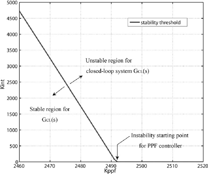
Stability threshold curve for closed loop system according to PPF controller gain and integral controller gain.

For the other case where PPF controller’s gain is in the stable region, then K_PPF and K_int are directly proportional to each other with negative slope. The value was K_PPF / K_int = –0.006944. For example, As the integral controller gain K_int increased from K_int = 0 to K_int = 77. The instability threshold point of PPF controller was changed from K_PPF = 2491.5 slightly down to K_PPF = 2491.0.

In other words, if we choose suitable integral gain, then the effect of K_int can be negligible so that the stability of G_CL(s) is decided almost by that of PPF controller. The example for fixed K_int = 10 and change of K_PPF was given in next section.

The conclusions are that both gains of PPF and integral controllers are directly proportional with each other with negative slope in the stable region and the upper limit of the stability condition for closed-loop system is decided by PPF controller.

4. Simulation

To validate stability condition derived in Eq. (50), root locus analysis and software simulation were performed for tension values of 600[kgf], 800[kgf] and 1300[kgf].

4.1. Stability Condition Calculations

The only information for stability condition in Eq. (50) is DC gain matrix g. For example, the values of that for tension value of 600[kgf] was given as follows   

$$\mathbf{g}=\left[\begin{array}{l}\text{0}\text{.2298 0}\text{.0983 0}\text{.0443 0}\text{.0224 0}\text{.0143}\\ \text{0}\text{.0983 0}\text{.1668 0}\text{.0741 0}\text{.0354 0}\text{.0224}\\ \text{0}\text{.0443 0}\text{.0741 0}\text{.1573 0}\text{.0741 0}\text{.0443}\\ \text{0}\text{.0224 0}\text{.0354 0}\text{.0741 0}\text{.1668 0}\text{.0983}\\ \text{0}\text{.0143 0}\text{.0224 0}\text{.0443 0}\text{.0983 0}\text{.2298}\end{array}\right]\times {10}^{-3}$$(62)

By solving Eqs. (49) and (50) with values of g, the value of controller gain K_PPF at which instability occurs was found to be K_PPF = 2491.5. In the same manner, the values were 3254.5 and 5116.9 for tension values of 800[kgf] and 1300[kgf] respectively. Figure 12 shows the change of determinant of stiffness matrix in Eq. (47) according to PPF controller gain. As the gain increased from zero, determinant decreased to zero and then became negative at the values of a K_PPF which was found using Eq. (50).

Fig. 12.

Change of determinant of stiffness matrix according to PPF controller gain.

4.2. Root Locus Analysis

The root locus analysis for the closed loop system, which include both PPF and integral controller in Eq. (53), was conducted to see the effect of integral controller to stability condition. For example, the root loci plot for tension value of 600[kgf] was given in Fig. 13, where the gain of PPF controller was increased from zero to 2500. The filter frequency ω_f of the PPF controllers was selected as 10 Hz and the integral controller gain K_int was set to 10, the value of which was also used in experiment in next section. Figure 13(a) shows that as the gain K_PPF increases, the eigenvalues initiated from the five poles of PPF controllers migrate along the negative real axis and then finally reached imaginary axis. To find exact value of K_PPF at which roots cross the imaginary axis, magnified root loci plot at the origin was shown in Fig. 13(b). The eigenvalues initiated from the poles of integral controller move toward the negative real axis and then encounter the poles from PPF controller. The root loci reverse their direction and cross the imaginary axis at the gain of K_PPF = 2491.5, and then continue to move into the right half plane. The value of gain K_PPF at which instability occurs was same as that derived in Eq. (50).

Fig. 13.

Root locus plot for tension 600[kgf]. (a) Root roci around PPF controller poles, (b) Root roci around integrator poles.

4.3. Software Simulation

In this simulation, strip vibration control with external periodic disturbance was simulated at various PPF filter frequencies. The transfer function matrix in Eq. (19) was used as the strip system, and the PPF controller in Eq. (36) was placed between the collocated input and the output pairs. The disturbance F_d(t) was given as:   

$$F_d(t)=sin(2\pi \cdot f_d\cdot t)$$(63)

where f_d is the frequency of disturbance, selected as 5 Hz assuming eccentricity of the rotating rollers frequency in real line. The filter frequency ω_f of the PPF controller was chosen as 1 Hz, 5 Hz, 10 Hz, and 20 Hz. The reason for selection is that 5 Hz is same as that of disturbance, between 5 Hz and 10 Hz the first natural frequency of strip is located. 1 Hz and 20 Hz is selected for comparison purpose.

Figure 14 shows the simulation results for PPF control with external periodic disturbance. y-axis represents magnitude of vibration and the x-axis represents PPF controller gain which is normalized to the value of K_PPF at which instability occurs. Figure 14(a) shows that the filter frequency of 1 Hz does not much contribute in vibration control because the frequency is far below that of disturbance nor natural frequency of strip. Figure 14(b) shows that when the filter frequency is matched to that of disturbance the control performance was better. Figure 14(c) shows 10 Hz has almost same performance as that of 5 Hz filter. As the filter frequency increased, there exist temporary increase in vibration as shown in Fig. 14(d). This may be explained by the existence of a more uncontrolled mode within the pass band frequency range of PPF filter. The phenomenon is also related to damping ratio of strip, so if strip is more highly damped then the magnitude of temporary overtshoot decreased. However without regardless of PPF filter frequency selection, maximum value of K_PPF at which instability occurs are same.

Fig. 14.

Change of magnitude of vibration for various PPF filter frequencies: (a) ω_f = 2π · 1[rad/sec], (b) ω_f = 2π · 5[rad/sec], (c) ω_f = 2π · 10[rad/sec], (d) ω_f = 2π · 20[rad/sec].

5. Experiments

5.1. Experimental Set-up

The strip vibration control system consists of electromagnet pairs, distance sensors, current amplifiers, and a controller. Five pairs of electromagnets were displaced, facing both sides of the strip as shown in Fig. 15. The electromagnets and sensors on both side of strip were denoted as top and bottom. Each electromagnet can exert a maximum force of 180 N at the excitation armatuer current of 6 A. The core material of electromagnet was SMC45C. The distance between the electromagnet and the strip was measured by laser sensors. Rotating vibrator was used to give forced vibration on the strip. A pulse-width modulation (PWM) current amplifier with a high-voltage DC link of 100 V was used to drive electromagnet current. By using the high-voltage PWM amplifier, the time delay owing to the electromagnet’s inductance was overcome, and the response time was improved. For the controller, Texas Instruments Digital Signal Processor F28335 was used. The controller contains an algorithm to generate the current reference signal to the PWM current amplifier. Bias current gives operating point of control current. Because electromagnet exert attractive force only, the electromanets shold be biased with constant postive current, which is called bias current.

Fig. 15.

Electromagnet and sensor arrangement of the vibration control system.

The hardware control block diagram was shown in Fig. 16, where D is the gap between the electromagnets on both side of strip and set to 30[mm]. The controller contain both PPF and intetral control algorithm. Discrete PPF control algorithm is implemented by using the one suggested by Rew et al.¹⁵⁾ as   

$$H_{PPF}(z)=\frac{U_{PPF}(z)}{Y(z)}=K_{PPF,D}\frac{z^{-1}}{1+P{z}^{-1}+Q{z}^{-2}}$$(64)

where   

$$\{\begin{array}{l}{K}_{PPF,D}=K_{PPF}\cdot {\omega }_f\sqrt{Q}\cdot sin\left({\omega }_f\sqrt{1-{\xi }_f^2}T\right)/{\sqrt{1-{\xi }_f^2}}_{,}\hfill \\ P=-2e^{-{\xi }_f{\omega }_{f}T}cos{\left({\omega }_f\sqrt{1-{\xi }_f^2}T\right)}_{,}\hfill \\ Q=e^{-2{\xi }_f{\omega }_{f}T}\hfill \end{array}$$(65)

where K_PPF,D is discrete controller gain and T is scan time of controller. And discrete integral control algorithm was used as   

$$H_{int}(z)=\frac{U_{int}(z)}{Y(z)}=-K_{int}\frac{T}{1+z^{-1}}$$(66)

Fig. 16.

Hardware control block diagram.

5.2. Stability Condition Test Results

Experiments for stability test were performed for tension values of 600[kgf], 800[kgf] and 1300[kgf]. Prior to gain increasing, rotating vibrator induced forced vibration on the strip with frequency of 5 Hz. All the electromagnets are biased with current of 0.65[A] and integral control was applied to make strip curvature flat. The filter frequencies of PPF controller was set to 5 Hz. And then gain of PPF controller was increased form zero until instability occurs.

Figure 17 shows the change of magnitude of vibration for tension value of 600 kgf for example. As the gain increases, the vibration get reduced and then break-out happened as shown in Fig. 17(a). To check the value of K_PPF at which instability occurs, magnified plot around instability point was shown in Fig. 17(b), which shows that when the stability condition was lost, strip deviated from operating point and accelerated to the electromagnet rapidly. The gain values where instability occurs are around 2650–2700. In the same manner, the change of magnitude of vibration until instability occur are plotted for tension values of 800[kgf] and 1300[kgf] in Fig. 18. Due to the stiffening effect of tension, induced forced vibration was not as large as that of 600[kgf]. However, we found that the gain at which instability occurs also increased as tension increased.

Fig. 17.

Experimental result for stability condition. (a) Change of magnitude of vibration for tension value of 600 kgf, (b) Magnitude plot around instability point.

Fig. 18.

Experimental results for change of vibration magnitude according to PPF gain.

For the various filter frequencies of PPF controller, the value of K_PPF at which instability occurs are listed in Table 3. which shows that experiments results are well agreed with that of calculation.

Table 3.Gain of PPF controller at which instability occurs.

	PPF Filter frequency	KPPF
		600[kgf]	800[kgf]	1300[kgf]
Calculation	5–20 [Hz]	2491	3254	5117
Experiments	5 [Hz]	2632	3369	5265
	10 [Hz]	2527	3264	4949
	15 [Hz]	2632	3159	4843
	20 [Hz]	2424	3161	4742
	30 [Hz]	2421	3053	4843

Finally, Fig. 19 shows performance of vibration and flatness control using PPF and integrator controller. Fig. 19(a) depicts on-off test result and Fig. 19(b) shows the corrected flatness of strip. The result shows that proposed controller work well for both vibration and flatness control at the same time.

Fig. 19.

Experimental results for vibration and flatness control performance using PPF with integration control. (a) Magnitude of vibration, (b) Flatness correction.

6. Conclusion

In this paper, analytical model based PPF controller gain decision method for active vibration and flatness control of a strip was established. Three dimensional FEM model and Krylov subspace technique was used to develop mathematical model of strip and system order reduction respectively. Stability condition for decentralized MIMO system including both PPF controller and integration controller was studied. Major findings are concluded as follows.

(1) DC gain concept was introduced to derive PPF controller stability condition for MIMO multi-degree-of-freedom system. By using the DC gain concept, higher order multi modal system was reduced to equivalent single-degree-of-freedom system. It reduced computation matrix size, PPF controller gain can be found easily by using the DC simple 5 × 5 DC gain matrix.

(2) Among the three design parameters of PPF controller, damping ratio and filter frequency has no concern with stability, the gain is only design parameter to decide. Gain can be calculated analytically based on strip model. so no trial and error is needed. it is very efficient when compared to model-less control such as PID or PD controller where design parameters are at least two or three.

(3) From the FEM model of strip we found that tension produces a stiffening effect and considerably increases the natural frequencies of the strip. DC gain of strip is inversely proportional to the square of natural frequency. So as tension increased, the DC gain of the strip was reduced. For this reason gain of PPF controller can be extended to higher value according to the increased tension value.

(4) By investigating the roci of eigenvalues, the stability threshold curve was obtained for the closed loop system which include both PPF and integral control loop. Both gains of PPF and integral controllers are directly proportional with each other with negative slope in the stable region. And the upper limit of the stability condition for closed-loop system is decided by PPF controller.

(5) Although the derivation procedure is complicated, the only information needed for PPF controller is simple 5 × 5 DC gains matrix of the strip. Usually the processing time of a coil in CGL is about 15 to 30 minute before next coil reached. It is enough time to calculate DC gain matrix online. Otherwise, DC gain matrix can be calculated beforehand and stored in a Database. Based on either method, on-line application can be possible.

References

• 1)   T.  Masui,  Y.  Kaseda and  K.  Ando: ISIJ Int., 31 (1991), 262.
• 2)  L. LinJian, Y.-H. Yan, X.-H. Guo and Y.-Q. Wang: ISIJ Int., 52 (2012), 1072.
• 3)   K.-J.  Yang,  K.-S.  Hong and  F.  Matsuno: J. Sound Vib., 273 (2004), 1007.
• 4)   S.  Morii,  A.  Inoue,  N.  Kawada,  H.  Suemori and  K.  Tsukuda: MHI. Tech. Rev., 32 (1995), 122.
• 5)   A.  Inoue,  H.  Fujioka,  S.  Morii and  M.  Komori: Trans. Jpn. Soc. Mech. Eng., 74 (2008), 2878.
• 6)   O.  Bruls and  J.-C.  Golinval: NATO Rev., 103 (2003), 325.
• 7)   M. I.  Friswell and  D. J.  Inman: Smart Mater. Struct., 8 (1999), 285.
• 8)   D.  Ramaswamy and  J.  White: Proc. Int. Conf. Modeling and Simulation of Microsystems, (2001), 27.
• 9)   Z.  Bai,  D.  Bindel,  J.  Clark,  J.  Demmel,  K. S. J.  Pister and  N.  Zhou: Proc. Int. Conf. Modeling and Simulation of Microsystems, (2001), 31.
• 10)   M. J.  Bals: J. Optimiz. Theory Appl., 25 (1978), 415.
• 11)   B.  Salimbahrami and  B.  Lohmann: Linear Algebra. Appl., 415 (2006), 385.
• 12)   R.  Eid,  B.  Salimbahrami,  B.  Lohmann,  E. B.  Rudnyi and  J. G.  Korvink: Sensor. Mater., 19 (2007), 149.
• 13)   C. J.  Goh and  T. K.  Caughey: Int. J. Control, 41 (1985), 787.
• 14)   D. J.  Inman: Phil. Trans. R. Soc. Lond. A, 359 (2001), 205.
• 15)   K.-H.  Rew,  J.-H.  Han and  I.  Lee: J. Intel. Mat. Syst. Str., 13 (2008), 13.