A New Model for the Prediction of Evolution of the Residual Stresses in Tension Leveling

Abstract

The shape defects such as edge waves and center buckles may be formed in the rolled strip, since rolling can easily produce non-homogenous elongation across the strip width. The main purpose of tension leveling is to cure such defects by eliminating the differences in elongation and thus eliminating the residual stresses. In this paper, a new model is presented for the prediction of the evolution of the residual stress distribution in the strip undergoing tension leveling. The model consists of an analytic model for the prediction of the strip curvature at each roll, the residual stress distribution along the width of the strip, and the roll force at each roll. The prediction accuracy of the proposed model is examined through comparison with the predictions from a finite element model.

1. Introduction

During rolling, elongation of a fiber may vary across the strip width, due to the non-uniform nature of plastic deformation, heat transfer, and phase transformation that the strip experiences. Consequently, a substantial level of residual stresses may manifest in the product, which would often accompany shape defects such as edge waves and center buckles. Tension leveling is performed to drastically reduce the magnitude of such residual stresses. During tension leveling, bending and tension are applied simultaneously, in such a way that the shorter (the longer) fiber would receive greater (smaller) elongation, so that elongation may eventually become uniform across the strip width. One of the most important issues in such a practice is, naturally, how to optimize the process conditions so as to reduce the residual stresses effectively, and it is in this regard that a sound mathematical model is desired which is capable of precisely predicting the evolution of the residual stresses throughout the process.

A classical model for predicting fiber elongation is due to Kinnavy¹⁾ in which dimensionless factors α and β are introduced which represent the contribution of stretching and the contribution of bending moment to total strain, respectively. However, a sound approach regarding proper selection of these values is yet to be developed. The model proposed by Misaka and Masui,²⁾ which is developed on the basis of experimental results, is widely used for process control.³⁾ Similar models are proposed by Hattori et al.,⁴⁾ and also, by Hibino.⁵⁾ The accuracy of their empirical equation for the calculation of bending curvature, which is vital for sound prediction of the evolution of residual stresses, however, may have to be examined for a wide range of process conditions.

In this paper, we present a new model for the prediction of the evolution of the residual stresses. A detailed description of the model is given, with emphasis on the analysis of the strip curvature. The prediction accuracy of the proposed model is examined through comparison with the predictions from a series of finite element simulation.

2. Basic Equations

The strip processed by tension leveling, illustrated in Fig. 1, is thin and wide. Therefore, we may assume that the normal stress acting across the strip thickness is negligible. Also, the plane strain condition would be applicable across the strip width. Let x, y, and z denote longitudinal direction, normal (thickness) direction and transverse (width) direction, respectively. Then   

$${\sigma }_y=d{\sigma }_y=0$$(1)

  

$$d{\mathit{\epsilon }}_z=d{\mathit{\epsilon }}_z^e+d{\mathit{\epsilon }}_z^p=0$$(2)

From the general Hooke’s law, we obtain   

$$d{\mathit{\epsilon }}_y^e=-\frac{\nu }{E}\left(d{\sigma }_x+d{\sigma }_z\right)$$(3)

  

$$d{\sigma }_x=\frac{E}{1-{\nu }^2}\left(d{\mathit{\epsilon }}_x^{}-d{\mathit{\epsilon }}_x^p-\nu d{\mathit{\epsilon }}_z^p\right)$$(4)

  

$$d{\sigma }_z=\frac{E}{1-{\nu }^2}\left(\nu d{\mathit{\epsilon }}_x^{}-d{\mathit{\epsilon }}_z^p-\nu d{\mathit{\epsilon }}_x^p\right)$$(5)

Note that the longitudinal strain increment may be expressed by   

$$d{\mathit{\epsilon }}_x=d\kappa y+d{\mathit{\epsilon }}_c\hspace{0.17em}$$(6)

where dκ is the increment of strip curvature, y is the distance from the strip center, and dε_c is the longitudinal strain increment at the strip center.

Fig. 1.

Tension leveling, a schematic view (a) the region where the strip undergoes plastic deformation while passing through a series of idle rolls placed on the top and bottom surfaces of the strip, (b) the front end of the strip which moves with the prescribed velocity, (c) the back end of the strip where tension is applied.

From Eqs. (4) and (6), we obtain   

$$d{\sigma }_x=\frac{E}{1-{\nu }^2}\left(d\kappa y+d{\mathit{\epsilon }}_c\left(z\right)-d{\mathit{\epsilon }}_x^p-\nu d{\mathit{\epsilon }}_z^p\right)$$(7)

The increment of the y-average longitudinal stress may then be defined by   

$$d{\overline{\sigma }}_x\left(z\right)=\frac{1}{t}{\int }_{\hspace{0.17em}-t/2}^{\hspace{0.17em}t/2}d{\sigma }_x\left(y,z\right)dy=C_{1}d\kappa +C_{2}d{\mathit{\epsilon }}_c\left(z\right)+C_3$$(8)

where t denotes the strip thickness, and   

$$C_1=\frac{1}{t}{\int }_{\hspace{0.17em}-t/2}^{\hspace{0.17em}t/2}\frac{E}{1-{\nu }^2}ydy\hspace{0.17em}$$(9)

  

$$C_2=\frac{1}{t}{\int }_{\hspace{0.17em}-t/2}^{\hspace{0.17em}t/2}\frac{E}{1-{\nu }^2}dy$$(10)

  

$$C_3=-\frac{1}{t}{\int }_{\hspace{0.17em}-t/2}^{\hspace{0.17em}t/2}\frac{E}{1-{\nu }^2}\left(d{\mathit{\epsilon }}_x^p+\nu d{\mathit{\epsilon }}_z^p\right)dy$$(11)

Also, in order for the applied tension to remain constant during leveling, the following condition should be satisfied.   

$${\int }_{\hspace{0.17em}-w/2}^{\hspace{0.17em}w/2}d{\overline{\sigma }}_x\left(z\right)dz=0$$(12)

From Eqs. (8) and (12), the increment of the z-average longitudinal strain at the strip center is given by   

$$d{\overline{\mathit{\epsilon }}}_c=\frac{1}{w}{\int }_{\hspace{0.17em}-w/2}^{\hspace{0.17em}w/2}d{\mathit{\epsilon }}_c\left(z\right)dz=-\frac{{\overline{C}}_{1}d\kappa +{\overline{C}}_3}{{\overline{C}}_2}$$(13)

where   

$${\overline{C}}_i=\frac{1}{w}{\int }_{\hspace{0.17em}-w/2}^{\hspace{0.17em}w/2}{C}_{i}dz$$(14)

The increment of the y-average longitudinal stress may be approximated by   

$$d{\overline{\sigma }}_x\left(z\right)=\overline{E}\left(d{\overline{\mathit{\epsilon }}}_c^{}-d{\mathit{\epsilon }}_c^{}(z)\right)$$(15)

where $\overline{E}$ denotes y-average Young’s modulus.

It follows from Eqs. (8), (13), and (15) that   

$$d{\mathit{\epsilon }}_c\left(z\right)=-\frac{\left(\frac{{\overline{C}}_1}{{\overline{C}}_2}\overline{E}+C_1\right)d\kappa +\frac{\overline{E}}{{\overline{C}}_2}{\overline{C}}_3+C_3}{C_2+\overline{E}}$$(16)

  

$$\begin{array}{c}d{\overline{\sigma }}_x\left(z\right)=\left[C_1-\frac{C_2}{C_2+\overline{E}}\left(\frac{{\overline{C}}_1}{{\overline{C}}_2}\overline{E}+C_1\right)\right]d\kappa \\ -\frac{C_2}{C_2+\overline{E}}\frac{\overline{E}}{{\overline{C}}_2}{\overline{C}}_3-\left(\frac{C_2}{C_2+\overline{E}}-1\right)C_3\end{array}$$(17)

We may divide cross-sectional plane of the strip into many small elements, as shown in Fig. 2. Let l = 1, 2, …, q denote the number of a vertical segment and let m = 1, 2, …, r denote the number of a parallel segment. Then, we may represent any parameter, say *, associated with an element, by (*)_lm. Also, we may represent the value of * evaluated at a vertical segment by (*)_l. Then, Eqs. (4), (5), (6), (16)–(17) may be approximated by   

$${\left(d{\mathit{\epsilon }}_c\right)}_l=-\frac{\left[\frac{{\overline{C}}_1^{*}}{{\overline{C}}_2^{*}}\overline{E}+{\left(C_1\right)}_l\right]d\kappa +\frac{\overline{E}}{{\overline{C}}_2^{*}}{\overline{C}}_3^{*}+{\left(C_3\right)}_l}{{\left(C_2\right)}_l+\overline{E}}$$(18)

  

$${\left(d{\mathit{\epsilon }}_x\right)}_{lm}=d\kappa {\left(y\right)}_m+{\left(d{\mathit{\epsilon }}_c\right)}_l\hspace{0.17em}$$(19)

  

$${\left(d{\overline{\sigma }}_x\right)}_l={\left(C_1\right)}_{l}d\kappa +{\left(C_2\right)}_l{\left(d{\mathit{\epsilon }}_c\right)}_l+{\left(C_3\right)}_l$$(20)

  

$${\left(d{\sigma }_x\right)}_{lm}=\frac{E}{1-{\nu }^2}\left[{\left(d{\mathit{\epsilon }}_x^{}\right)}_{lm}-{\left(d{\mathit{\epsilon }}_x^p\right)}_{lm}-\nu {\left(d{\mathit{\epsilon }}_z^p\right)}_{lm}\right]$$(21)

  

$${\left(d{\sigma }_z\right)}_{lm}=\frac{E}{1-{\nu }^2}\left[\nu {\left(d{\mathit{\epsilon }}_x^{}\right)}_{lm}-{\left(d{\mathit{\epsilon }}_z^p\right)}_{lm}-\nu {\left(d{\mathit{\epsilon }}_x^p\right)}_{lm}\right]$$(22)

where   

$${\left(C_1\right)}_l=\frac{1}{t}\sum _{m=1}^r\frac{E}{1-{\nu }^2}{\left(y\right)}_m\mathrm{\Delta }y\hspace{0.17em}$$(23)

  

$${\left(C_2\right)}_l=\frac{1}{t}\sum _{m=1}^r\frac{E}{1-{\nu }^2}\mathrm{\Delta }y$$(24)

  

$${\left(C_3\right)}_l=-\frac{1}{t}\sum _{m=1}^r\frac{E}{1-{\nu }^2}\left[{\left(d{\mathit{\epsilon }}_x^p\right)}_{lm}+\nu {\left(d{\mathit{\epsilon }}_z^p\right)}_{lm}\right]\mathrm{\Delta }y$$(25)

  

$${\overline{C}}_{1,2,3}^{*}=\frac{1}{w}\sum _{l=1}^q{\left(C_{1,2,3}\right)}_l\mathrm{\Delta }z$$(26)

Fig. 2.

(a) strip geometry, (b) mesh representing the cross-sectional plane of the strip

3. Calculation of the Plastic Strain Increment

Using the radial return algorithm,⁶⁾ the plastic strain increments may be calculated, as follows:

Define   

$$R^{TL}=\sqrt{{\sigma }_{ij}^{\text{'}TL}{\sigma }_{ij}^{\text{'}TL}}$$(27)

  

$$R^{N+1}=\sqrt{{\sigma }_{ij}^{\text{'}N+1}{\sigma }_{ij}^{\text{'}N+1}}=\sqrt{\frac{2}{3}}{Y}^{N+1}$$(28)

where Y^N+1 and ${\sigma }_{ij}^{\text{'}N+1}$ denote the flow stress and the deviatoric stress tensor at time step N+1, respectively, and   

$${\sigma }_{ij}^{\text{'}TL}={\sigma }_{ij}^{\text{'}N}+2\mu d{\mathit{\epsilon }}_{ij}^{\text{'}}$$(29)

where $d{\mathit{\epsilon }}_{ij}^{\text{'}}$ denotes the deviatoric strain increment tensor. Figure 3 graphically shows the definition of ${\sigma }_{ij}^{\text{'}TL}$ .

Fig. 3.

A graphical representation of the radial return algorithm.

From Eqs. (1), (2), (3), (4), (5) and the incompressibility of plastic deformation, it may be shown that   

$$d{\mathit{\epsilon }}_x^{\text{'}}=\frac{2-\nu }{3\left(1-\nu \right)}d{\mathit{\epsilon }}_x+\frac{1-2\nu }{3\left(1-\nu \right)}d{\mathit{\epsilon }}_x^p+\frac{1-2\nu }{3\left(1-\nu \right)}d{\mathit{\epsilon }}_z^p$$(30)

  

$$d{\mathit{\epsilon }}_y^{\text{'}}=-\frac{1+\nu }{3\left(1-\nu \right)}d{\mathit{\epsilon }}_x^{}-\frac{2\left(1-2\nu \right)}{3\left(1-\nu \right)}d{\mathit{\epsilon }}_x^p-\frac{2\left(1-2\nu \right)}{3\left(1-\nu \right)}d{\mathit{\epsilon }}_z^p$$(31)

  

$$d{\mathit{\epsilon }}_z^{\text{'}}=-\frac{1-2\nu }{3\left(1-\nu \right)}\left(d{\mathit{\epsilon }}_x^{}-d{\mathit{\epsilon }}_x^p-d{\mathit{\epsilon }}_z^p\right)$$(32)

The plastic strain increments are then calculated from   

$$d{\mathit{\epsilon }}_{ij}^p=\{\begin{array}{cc}\frac{R^{TL}-R^{N+1}}{2\mu }\frac{{\sigma }_{ij}^{\text{'}TL}}{R^{TL}}& if\hspace{0.17em}\hspace{0.17em}{R}^{TL}>R^{N+1}\\ 0& if\hspace{0.17em}\hspace{0.17em}{R}^{TL}<R^{N+1}\end{array}$$(33)

Equation (33) indicates that if plastic deformation occurs, the plastic strain increments may be expressed as   

$$d{\mathit{\epsilon }}_x^p=C{\sigma }_x^{\text{'}TL}$$(34)

  

$$d{\mathit{\epsilon }}_z^p=C{\sigma }_z^{\text{'}TL}$$(35)

where   

$$C=\frac{\sqrt{{\left({\sigma }_x^{\text{'}TL}\right)}^2+{\left({\sigma }_y^{\text{'}TL}\right)}^2+{\left({\sigma }_z^{\text{'}TL}\right)}^2}-\sqrt{\frac{2}{3}}Y}{2\mu \sqrt{{\left({\sigma }_x^{\text{'}TL}\right)}^2+{\left({\sigma }_y^{\text{'}TL}\right)}^2+{\left({\sigma }_z^{\text{'}TL}\right)}^2}}$$(36)

From Eqs. (30), (31), (32), (33), and Eqs. (34)–(35), it is clear that the plastic strain increments are dependent on the longitudinal strain increment and also on themselves. Namely,   

$$d{\mathit{\epsilon }}_x^p-f_x\left(d{\mathit{\epsilon }}_x^{},d{\mathit{\epsilon }}_x^p,d{\mathit{\epsilon }}_z^p\right)=0$$(37)

  

$$d{\mathit{\epsilon }}_z^p-f_z\left(d{\mathit{\epsilon }}_x^{},d{\mathit{\epsilon }}_x^p,d{\mathit{\epsilon }}_z^p\right)=0$$(38)

Equations (37)–(38) may be solved for the plastic strain increments by using an iterative solution technique such as Newton-Rhapson method.

The following procedure may then be taken to predict the change of the residual stress distribution in a cross-section of the strip during tension leveling.

1) Read initial stress distribution and initial curvature.

2) Read the increment of the strip curvature dκ.

3) Assume that the plastic strains are equal to zero, $d{\mathit{\epsilon }}_x^p=d{\mathit{\epsilon }}_z^p=0$ .

4) Calculate the increment of the strain at center, dε_c from Eq. (18).

5) Calculate the increment of the longitudinal strain, dε_x from Eq. (19).

6) Calculate the increments of the deviatoric strain, $d{\mathit{\epsilon }}_{x,y,z}^{\text{'}}$ from Eqs. (30), (31), (32).

7) Calculate the increments of the plastic strain, $d{\mathit{\epsilon }}_{ij}^p$ from Eq. (33).

8) Repeat from 4) to 7) until the convergence.

9) If the increments of the plastic strain converge, calculate the increment of the stresses and the average increment of the longitudinal stress, dσ_x, dσ_z and $d{\overline{\sigma }}_x$ from Eqs. (20), (21), and (22).

10) Update the stresses and the average longitudinal stress, σ_x, σ_z, and $\overline{\sigma }{}_x$ .

11) Repeat from 2) to 10), until the strip section completely passes through the tension leveling process.

4. An Approximate Model for the Prediction of the Strip Curvature

As may be seen in Eq. (6), sound prediction of the change in the curvature of the strip during tension leveling is a prerequisite for precise prediction of the evolution of the residual stresses in it. Let us consider a strip segment between two adjacent rolls, which constitutes a part of the whole strip, as shown in Fig. 4(a). Three assumptions are adopted for the prediction of the strip curvature, as follows. (1) Change in the sign of the curvature occurs at the mid-point between two rolls. (2) The deflection of the strip at the mid-point is one-half of the compression depth of the roll. (3) The tensile force is acting along the center line of the strip.

Fig. 4.

(a) process geometry (b) the free body diagram for one half of the strip between two adjacent rolls (c) the free body diagram showing the variation of the bending moment in the strip.

As may be seen from Fig. 4(b), the maximum moment is given by   

$$M_n=\frac{P_{n}L}{2}-F_0{y|}_{L/2}$$(39)

where n denotes strip segment number, P_n denotes the shear force acting in the strip segment, F₀ denotes the applied tension, and ${y|}_{L/2}$ denotes the deflection of the strip at the mid-point of the strip segment, as shown in Fig. 4(b).

Also from Fig. 4(c), the moment is given by,   

$$M\left(x\right)=M_n-P_{n}x+F_{0}y\left(x\right)$$(40)

From the beam theory, we have   

$$\frac{M_n}{EI}=\frac{1}{{\rho }_n}\hspace{0.17em}={\kappa }_n$$(41)

  

$$M\left(x\right)=EI\frac{d^{2}y}{d{x}^2}$$(42)

By substituting Eqs. (39) into (40), and using Eqs. (41) and (42), we obtain a second order differential equation, which may be expressed by   

$$y\text{'}\text{'}-\frac{F_0}{EI}y=\frac{1}{{\rho }_n}\left(1-\frac{2x}{L}\right)-\frac{2}{L}\frac{F_0}{EI}{y|}_{L/2}x$$(43)

Solving Eq. (43) using the boundary conditions   

$$y=y\text{'}=0\hspace{0.17em}\hspace{0.17em}\hspace{0.17em}\hspace{0.17em}\hspace{0.17em}at\hspace{0.17em}\hspace{0.17em}x=0$$(44)

we obtain   

$$\begin{array}{c}y\left(x\right)=\frac{EI}{F_0{\rho }_n}cosh\left(\sqrt{\frac{F_0}{EI}}x\right)\hfill \\ -\frac{2}{L}\frac{EI}{F_0}\sqrt{\frac{EI}{F_0}}\left(\frac{1}{{\rho }_n}+\frac{F_0}{EI}{y|}_{L/2}\right)sinh\left(\sqrt{\frac{F_0}{EI}}x\right)\\ -\frac{EI}{F_0{\rho }_n}+\frac{2}{L}\frac{EI}{F_0}\left(\frac{1}{{\rho }_n}+\frac{F_0}{EI}{y|}_{L/2}\right)x\hfill \end{array}$$(45)

This solution contains two unknowns of ρ_n and ${y|}_{L/2}$ . The relation between them may be derived by noting that ${y|}_{L/2}$ is y(x) at x=L/2. The result being   

$${y|}_{L/2}=\frac{L{A}_{}}{2{\rho }_n}$$(46)

where   

$$A_{}=\sqrt{\frac{EI}{F_0}}\left(\frac{cosh\left(\sqrt{\frac{F_0}{EI}}\frac{L}{2}\right)}{sinh\left(\sqrt{\frac{F_0}{EI}}\frac{L}{2}\right)}-\sqrt{\frac{EI}{F_0}}\frac{2}{L}\right)$$(47)

According to the assumptions (1) and (2), the curvature at an end of the strip segment should be same as that at the other end, while they are opposite in sign. From assumption (3) and Eq. (46), the curvature is found to be   

$${\kappa }_n=\frac{1}{{\rho }_n}=\frac{{\delta }_n}{LA}$$(48)

where δ_n is the compression depth.

It is clear from Eqs. (45), (46), (47), (48) that the effect of the compression depth and tensile force on the deflection and the curvature at any point in the strip is given by   

$$\begin{array}{c}y\left(x\right)=\frac{EI}{F_0}{\kappa }_{n}cosh\left(\sqrt{\frac{F_0}{EI}}x\right)\hfill \\ -\frac{2}{L}\frac{EI}{F_0}\sqrt{\frac{EI}{F_0}}\left({\kappa }_n+\frac{F_0}{EI}\frac{{\delta }_n}{2}\right)sinh\left(\sqrt{\frac{F_0}{EI}}x\right)\\ -\frac{EI}{F_0}{\kappa }_n+\frac{2}{L}\frac{EI}{F_0}\left({\kappa }_n+\frac{F_0}{EI}\frac{{\delta }_n}{2}\right)x\hfill \end{array}$$(49)

  

$$y\text{'}\text{'}\left(x\right)=\frac{F_0}{EI}y\left(x\right)+{\kappa }_n\left(1-\frac{2x}{L}\right)-\frac{2}{L}\frac{F_0}{EI}\left(\frac{{\delta }_n}{2}\right)x$$(50)

Note that the curvature, given by Eq. (48), may differ at a different strip segment, due to possible differences either in the length L or in the compression depth δ. Consequently, the curvature is in general discontinuous at the junction of two adjacent strip segments, which is, at the point touching a roll. However, it may be assumed that the average value of the curvature predicted from each of the two strip segments would closely represent the actual curvature at that point.

5. An Approximate Model for the Prediction of the Roll Force

As shown in Fig. 4(b), the shear force is given by   

$$P_n=\frac{2}{L}\left(M_n+F_0\frac{{\delta }_n}{2}\right)$$(51)

The bending moment is given by   

$$M={\int }_{\hspace{0.17em}-\frac{t}{2}}^{\hspace{0.17em}\frac{t}{2}}\sigma ydA=2\left[{\int }_{\hspace{0.17em}0}^{\hspace{0.17em}{t}_1}E\frac{y}{\rho }ywdy+{\int }_{\hspace{0.17em}{t}_1}^{\hspace{0.17em}\frac{t}{2}}{\sigma }_{Y}ywdy\right]$$(52)

where t₁ denotes the half thickness of the elastic layer in the strip.

It may be shown that   

$$M_n=\frac{{\sigma }_{Y}w{t}^2}{4}\left(1-\frac{1}{3{\gamma }_n^2}\right)$$(53)

where   

$${\gamma }_n=\frac{t/2}{t_1}=\frac{{\kappa }_{n}tE}{2{\sigma }_Y}$$(54)

It follows that   

$$P_n=\frac{2}{L}\left(\frac{{\sigma }_{Y}w{t}^2}{4}\left(1-\frac{1}{3{\gamma }_n^2}\right)+F_0\frac{{\delta }_n}{2}\right)$$(55)

The roll force acting on a roll is then simply the summation of the shear force acting at each of two adjacent strip segments which are in contact with the roll. Note that, as in the case of the curvature, the shear force may differ at a different strip segment, due to possible differences either in the length L or in the compression depth δ.

6. A Finite Element Model

A finite element model for the analysis of 3D non-steady elastic-plastic deformation, which is described in detail in the reference,⁷⁾ is used for the examination of the prediction accuracy of the proposed model. Initially, the prescribed tension is applied to the back end of the strip while the front end is attached to a frictionless, flat die, as illustrated in Fig. 1-(b), and all the upper rolls are in contact with the strip. The first step of FE simulation is the upward movement of the lower rolls until the prescribed compression depth is achieved. The second step is to pull the flat die with a prescribed velocity, until the steady-state is reached regarding stress distributions in the deformation zone.

For the validation of the present model, tension leveling with three rolls is investigated, which is described in Fig. 5. The strip subject to tension leveling is assumed to be 1.0 mm thick and 800 mm wide. Also assumed are; Young’s modulus of the strip is 200 GPa, Poisson’s ratio is 0.3, and the yield strength of the strip is 400 MPa, the prescribed tension at the back end of the strip is 200 MPa, and the prescribed velocity of the flat die is 5000 mm/sec. The intermeshes considered are 0.7 mm and 1.5 mm.

Fig. 5.

Tension leveling with three rolls, process geometry.

In order to eliminate the effect of the mesh size as well as the time step size on the solution accuracy, a series of numerical tests were conducted. The mesh selected from these tests, is found to be one having 12 elements across the half width of the strip, 6 elements across the thickness of the strip, while the length of each element along the moving direction being 1/60 of the roll diameter, which amounts to 0.667 mm. In order to ensure achieving the steady-state stress distributions, the strip length is selected to be 400 mm, five times longer than the roll pitch, which leads to using 600 elements across the length of the strip. For the time step size, 0.000012 second was chosen. With this time step size, simulation requires about 5000 time steps.

7. Results and Discussion

As may be seen in Figs. 6 and 7, the predicted strip curvature is in excellent agreement with the predictions from FEM, either when 0.7 mm intermesh is applied or when 1.5 mm intermesh is applied. The predicted progressive reduction in the residual stress level as the strip passes through the roll gaps, as well as the predicted roll force, are also found to match precisely the predictions from FEM, as illustrated in Figs. 8, 9, 10.

Fig. 6.

The strip curvature, for 0.7 mm intermesh (three rolls).

Fig. 7.

Strip curvature, for 1.5 mm intermesh (three rolls).

Fig. 8.

Evolution of the residual stress distribution, for 0.7 mm intermesh (three rolls).

Fig. 9.

Evolution of the residual stress distribution, for 1.5 mm intermesh (three rolls).

Fig. 10.

Roll force, for 1.5 mm intermesh (three rolls).

Verification is also performed for a more complex process geometry, which involves six rolls with different roll diameters, as shown in Fig. 11. Note that the process consists of ‘stretching unit’, and ‘anti-cambering unit’. The process conditions are, as summarized in Table 1, as follows. The stretching unit consists of three rolls, with the diameter of each roll being 30 mm (roll no. 1), 30 mm (roll no. 2), and 80 mm (roll no. 3), respectively. The distances between two adjacent rolls are, L₁ = 30 mm, and L₂ = 80 mm. The anti-cambering unit consists of three rolls, with the diameter of each roll being 80 mm (roll no. 4), 40 mm (roll no. 5), and 80 mm (roll no. 6), respectively. The distances between two adjacent rolls in this unit are all 42.5 mm. The distance between the stretching unit and the anti-cambering unit is D = 100 mm. The intermesh of the stretching unit as well as that of the anti-cambering unit is 0.4 mm. The strip thickness, width and the material properties are the same as those used in tension leveling with three rolls. It is assumed that the yield strength of the strip is 400 MPa, the prescribed tension at the back end of the strip is 200 MPa, and the prescribed velocity of the flat die is 5000 mm/sec.

Fig. 11.

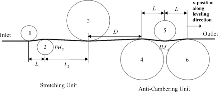
Process geometry, industrial tension leveling.

Table 1. Process condition, an industrial tension leveling process.

Stretching unit	L1 (mm)	30.0
	L2 (mm)	80.0
	Roll 1 diameter (mm)	30.0
	Roll 2 diameter (mm)	30.0
	Roll 3 diameter (mm)	80.0
	Intermesh IMs (mm)	0.4
Between units	D (mm)	100.0
Anti-cambering unit	L (mm)	42.5
	Roll 4 diameter (mm)	80.0
	Roll 5 diameter (mm)	40.0
	Roll 6 diameter (mm)	80.0
	Intermesh IMA (mm)	0.4

Regarding the FE mesh used, the same mesh as used in the investigation of tension leveling with three rolls is used. Namely, 12 elements across the half width of the strip and 6 elements across the thickness of the strip are used, while the length of each element along the moving direction is 0.667 mm. In order to ensure achieving the steady-state stress distributions, the strip length is selected to be as great as 800 mm.

The predicted strip curvature, the predicted progressive reduction of residual stress level both in the stretching unit and in the anti-cambering unit and the predicted roll force are in excellent agreement with the predictions from FEM, as shown in Figs. 12, 13, 14, 15.

Fig. 12.

Strip curvature, industrial tension leveling.

Fig. 13.

Evolution of the residual stress distributions, industrial tension leveling, the stretching unit.

Fig. 14.

Evolution of the residual stress distributions, industrial tension leveling, the anti-cambering unit.

Fig. 15.

Roll force, industrial tension leveling.

8. Concluding Remarks

Process setup and control in tension leveling is mainly practiced on the basis of an operator’s experience, as in many other steel processing lines in the mill. Definitely, a scientific approach is highly desired, for the purpose of improving the product quality and reducing the production cost. There are two pre-requisites to achieve this goal. One is the on-line capability of precisely predicting the residual stress distributions in the strip, and the other is the on-line capability of precisely predicting the evolutions of the residual stresses during tension leveling. In this paper, a new model is presented with regard to the latter. It is shown that the model’s prediction accuracy is comparable to that of FEM. Considering that approximately two CPU seconds are consumed when prediction is to be made using a personal computer, the model may play an important role in sound, automatic process setup and control in tension leveling.

Nomenclature

ε_ij = strain tensor

${\mathit{\epsilon }}_{ij}^e$ = elastic strain tensor

${\mathit{\epsilon }}_{ij}^p$ = plastic strain tensor

${\mathit{\epsilon }}_{ij}^{\text{'}}$ = deviatoric strain tensor

ε_c = longitudinal strain at the strip center

σ_ij = stress tensor

${\sigma }_{ij}^{\text{'}}$ = deviatoric stress tensor

σ_Y = yield strength

${\overline{\sigma }}_x^{}$ = y-average longitudinal stress

E = Young’s modulus (elastic modulus)

μ = shear modulus

I = moment of inertia of the strip

IM = intermesh of lower roll

v = Poisson’s ratio

κ = curvature of the strip

ρ = curvature radius of the strip

γ = ratio between the thickness of the strip and the thickness of the elastic part

δ = compression depth

L = distance between two rolls

t = thickness of the strip

w = width of the strip

References

• 1)   M. G.  Kinnavy: Iron Steel Eng., 49 (1972), 67.
• 2)   Y.  Misaka and  T.  Masui : J. Jpn. Soc. Technol. Plast., 17 (1976), 988.
• 3)   Y.  Kimura,  M.  Ueno and  Y.  Sodani: 44th MWSP Conf. Proc., Vol. XL, Materials & Processing Research Center, Orlando, (2002), 1011.
• 4)   S.  Hattori,  K.  Maeda,  T.  Matsushita,  S.  Murakami and  J.  Hata: J. Jpn. Soc. Technol. Plast., 28 (1987), 34.
• 5)   F.  Hibino : J. Jpn. Soc. Technol. Plast., 31 (1990), 208.
• 6)   R. D.  Krieg and  D. B.  Krieg: J. Pressure Vessel Tech., 90 (1977), 510.
• 7)   J. M.  Koo,  S. R.  Ryoo,  C. S.  Lee,  C. G.  Sun,  H. N.  Han and  S. M.  Hwang: ISIJ Int., 47 (2007), 1149.