Numerical Simulation of Molten Steel Flow and Inclusions Motion Behavior in the Solidification Processes for Continuous Casting Slab

Abstract

A three-dimensional numerical simulation of transient fluid flow field during the solidification process of casting mold has been developed to predict the solidification front capturing the inclusions and the distribution of the inclusions at the different location in the inner surface layer has been given out. The motion behavior of non-metallic inclusions which are more than 50 μm has been simulated and visually displayed. The results show the large inclusions and the small inclusions cluster at different location in the inner surface layer through numerical simulation, and the inclusion cluster at the quarter of the broad face through numerical simulation and experiment.

1. Introduction

The transport phenomena in the continuous casting processes for slab, billet and bloom caster is a hot topic in the past three decades. Solidification coupled with flow becomes more important since it affects the distribution of the element and discrete phase more obviously. A series of papers use different model to study the solidification of the continuous casting slab.^1,2,3,4) The enthalpy-porosity technique⁵⁾ which can couple the flow with heat transfer directly becomes the more popular method for deal with solidification coupled with flow. More attentions were paid to the coupled mathematical model on turbulent flow, heat transfer and mass transfer in the continuous casting process.^6,7) The numerical simulation has been used for the prediction of inclusion behavior, such as inclusion trajectory, inclusion removed in the RH,⁷⁾ tundish,^8,9,10,11) and casting mold.^12,13) But the inclusion behavior only focused on considering the influence of flow field on inclusion distribution and the removal effect. A lot of papers used trajectory model^13,14,15) to investigate inclusion behavior in the continuous casting mold. Some papers^13,16,17,18) have coupled the flow of the molten steel with removal and trajectory of inclusions in the mold and tundish. But there is few papers coupled solidification with flow and inclusions motion in the continuous casting mold. The distribution of the large inclusion at the different location in the shell can rarely been seen.

The distribution of the large inclusion in the slab will affect the quality of the slab. It’s more important for high surface quality requirements steel and high mechanical properties steel. So studying the distribution of the large inclusion in the shell becomes more important than before. This work presents a three-dimensional numerical simulation of transient fluid flow field during the solidification process of casting mold. Non-metallic inclusion motion behavior is simulated and visually displayed, and the non-metallic inclusion captured by the solidification front in the solidification process is a new feature in this work. The simulation data agree well with the experiment data.

2. Simulation Model

The simulation model divided into two models: the Solidification Model and Inclusions Capturing Model. The Solidification Model is a steady simulation model which provides the initial condition for the Inclusions Capturing Model, such as the temperature distribution, the flow state and the steel shell thickness distribution. However the Inclusions Capturing Model is a transient model which includes the simulation of the temperature, flow, solidification and inclusions capturing. The equations for continuity, Navier–Stokes, and turbulent kinetic energy and its dissipation rate are listed as follows.^19,20,21)

2.1. Assumptions in this Model

The following assumptions have been included in the present mathematical model for the complexity of the inclusion transfer phenomena during the solidification process of liquid steel.

(1) The molten steel is considered as steady and incompressible Newton flow.

(2) No considering the fluctuation of molten steel in mold. The top surface is covered with a protective slag layer which keeps the surface thermally insulated from the surroundings.

(3) The caster is perfectly vertical with respect to the gravitational field and the curvature of the strand is ignored.

(4) The non-metallic inclusions are spherical, and constant density of 3500 kg/m³ for inclusions is assumed.

(5) No considering the impact of small inclusion particles on collision growth during the solidification process of steel slab. The inclusions can’t influence fluid flow and heat transfer for their relatively low volume fraction in the molten steel.

(6) Only the evolution of latent heat due to solid liquid phase change is taken into account.

(7) Darcy’s law is applied as the flow resistance through the mushy zone.

2.2. Inclusions Capturing Model

2.2.1. Single-phase Mass Transport

  

$$\frac{\partial \rho }{\partial \text{t}}+\nabla \cdot \left(\rho \text{U}\right)=0$$(1)

Where ρ is density of molten steel in kg/m³, t is the time in s, U is velocity in m/s.

2.2.2. Momentum Transport

  

$$\frac{\partial }{\partial \text{t}}\left(\rho \text{U}\right)+\rho \text{U}\cdot \nabla \text{U}={\mu }_{\text{eff}}{\nabla }^2\text{U}-\nabla \text{p}-{\text{S}}_{\text{U}}$$(2)

Where p is the static pressure, μ_eff is the effective viscosity of the fluid steel, S_U is the momentum source.   

$${\mu }_{\text{eff}}=\mu +{\mu }_{\text{t}}$$(3)

  

$${\mu }_{\text{t}}={\text{c}}_{\mu }\frac{\rho {\text{K}}^2}{\mathit{\epsilon }}$$(4)

Where μ is viscosity of the liquid steel, where μ_t is the turbulent viscosity, K is the turbulent kinetic energy, and ε is turbulent energy dissipation, and c_μ is a constant, and its value is 0.09.

The enthalpy-porosity technique⁵⁾ treats the mushy region as a porous medium. The porosity in each cell is set equal to the liquid fraction in that cell. In fully solidified regions, the porosity is equal to U_cast.   

$${\text{S}}_{\text{U}}=\frac{\left(1-\text{f}\right)}{{\text{f}}^3+\text{e}}{\text{A}}_{\text{mush}}\left(\text{U}-{\text{U}}_{\text{cast}}\right)$$(5)

Where f is the liquid volume fraction defined in the Eq. (8), e is a small number (0.001) to prevent division by zero, A_mush is the mushy zone constant, and U_cast is the solid velocity due to the pulling of solidified material out of the domain.

2.2.3. Enthalpy Transport

The enthalpy of the material is computed as the sum of the sensible enthalpy h and the latent heat ΔH:   

$$\text{H}=\text{h}+\mathrm{\Delta }\text{H}$$(6)

  

$$\text{h}={\text{h}}_{\text{ref}}+{\int }_{{\text{T}}_{\text{ref}}}^{\text{T}}{\text{c}}_{\text{p}}\text{dT}$$(7)

h_ref=reference enthalpy

T_ref=reference temperature

c_p=specific heat at constant pressure

The liquid fraction f can be defined as:   

$$\text{f}=\{\begin{array}{c}0\cdots \left(\text{T}<{\text{T}}_{\text{solidus}}\right)\\ \frac{\text{T}-{\text{T}}_{\text{solidus}}}{{\text{T}}_{\text{liquidus}}-{\text{T}}_{\text{solidus}}}\cdots \\ 1\cdots (\text{T}>{\text{T}}_{\text{liquidus}})\end{array}({\text{T}}_{\text{solidus}}<T<{\text{T}}_{\text{liquidus}})$$(8)

  

$$\mathrm{\Delta }\text{H}=\text{f}\cdot {\text{H}}_{\text{latentHeat}}$$(9)

  

$$\frac{\partial }{\partial \text{t}}\left(\rho \text{H}\right)+\nabla \cdot \left(\rho \text{UH}\right)-\nabla \cdot \left({\text{k}}_{\text{eff}}\nabla \text{T}\right)=0$$(10)

k_eff is the effective thermal conductivity.   

$${\text{k}}_{\text{eff}}=\text{k}+{\text{k}}_{\text{t}}$$(11)

Where k is thermal conductivity, k_t is the turbulent thermal conductivity.

2.2.4. Transport Equations for the Standard k-ε Model

The turbulence kinetic energy K, and its rate of dissipation ε are obtained from the following transport equations:   

$$\frac{\partial }{\partial \text{t}}\left(\rho \text{K}\right)+\frac{\partial }{\partial {\text{x}}_{\text{j}}}\left(\rho {\text{KU}}_{\text{j}}\right)=\frac{\partial }{\partial {\text{x}}_{\text{j}}}\left[\left(\mu +\frac{{\mu }_{\text{t}}}{{\sigma }_{\text{K}}}\right)\frac{\partial \text{K}}{\partial {\text{x}}_{\text{j}}}\right]+{\text{G}}_{\text{K}}-\rho \mathit{\epsilon }$$(12)

  

$$\begin{array}{l}\frac{\partial }{\partial \text{t}}\left(\rho \mathit{\epsilon }\right)+\frac{\partial }{\partial {\text{x}}_{\text{j}}}\left(\rho \mathit{\epsilon }{\text{U}}_{\text{j}}\right)=\\ \frac{\partial }{\partial {\text{x}}_{\text{j}}}\left[\left(\mu +\frac{{\mu }_{\text{t}}}{{\sigma }_{\mathit{\epsilon }}}\right)\frac{\partial \mathit{\epsilon }}{\partial {\text{x}}_{\text{j}}}\right]+{\text{C}}_{1\mathit{\epsilon }}\frac{\mathit{\epsilon }}{\text{K}}{\text{G}}_{\text{k}}-{\text{C}}_{2\mathit{\epsilon }}\rho \frac{{\mathit{\epsilon }}^2}{\text{K}}\end{array}$$(13)

Where G_K represents the generation of turbulence kinetic energy due to the mean velocity gradients, defined as below:   

$${\text{G}}_{\text{K}}=-\rho \overline{{\text{U}}_{\text{i}}^{\prime }{\text{U}}_{\text{j}}^{\prime }}\frac{\partial {\text{U}}_{\text{j}}}{\partial {\text{x}}_{\text{i}}}$$(14)

And C_1ε, C_2ε, σ_K, σ_ε are constants. Given by Launder, B. E. and D. B. Spalding²²⁾ as below:   

$${\text{C}}_{1\mathit{\epsilon }}=1.44,\mathrm{\hspace{0.17em} }\hspace{0.17em}{\text{C}}_{2\mathit{\epsilon }}=1.92,\mathrm{\hspace{0.17em} }\hspace{0.17em}{\sigma }_{\text{K}}=1.0,\hspace{0.17em}\mathrm{\hspace{0.17em} }{\sigma }_{\mathit{\epsilon }}=1.3$$

2.2.5. Particle Force Balance

The movement of the inclusions is governed by the particle force balance equation defined as below:   

$$\frac{{\text{dU}}_{\text{p}}}{\text{dt}}=\frac{3}{4{\rho }_{\text{p}}{\text{d}}_{\text{p}}}{\text{C}}_{\text{D}}\rho \left|{\text{U}}_{\text{p}}-\text{U}\right|\left(\text{U}-{\text{U}}_{\text{p}}\right)+\frac{{\text{g}}_{\text{x}}\left({\rho }_{\text{p}}-\rho \right)}{{\rho }_{\text{p}}}+{\text{F}}_{\text{i}}$$(15)

  

$${\text{F}}_{\text{drag}}=\frac{3}{4{\rho }_{\text{p}}{\text{d}}_{\text{p}}}{\text{C}}_{\text{D}}\rho \left|{\text{U}}_{\text{p}}-\text{U}\right|\left(\text{U}-{\text{U}}_{\text{p}}\right)$$(16)

Where F_drag is the drag force per unit particle mass, F₁ is additional force per unit particle mass (Saffman force²³⁾ and Suction force caused by the concentration gradient²⁴⁾). C_D is dimensionless drag coefficient as a function of particle, as the approach of Crowe²⁵⁾ describing, C_D = (1 + 0.15 ${\text{Re}}_{\text{p}}^{0.687}$ ) 24/Re_p, Re_p is the particle Reynolds number, U is the fluid phase velocity in m/s, U_p is the particle velocity in m/s, ρ is the fluid density in kg/m³, ρ_p is the density of the particle in kg/m³, and d_p is the particle diameter in m.

Saffman force which caused by the uneven velocity distribution of the velocity boundary layer is defined as below:   

$${\text{F}}_{\text{s}}=1.62\mu \left(\text{U}-{\text{U}}_{\text{p}}\right)\sqrt{\frac{\partial \text{U}}{\partial {\text{x}}_{\text{i}}}}\frac{{\text{d}}_{\text{p}}^2}{\sqrt{\nu }}$$(17)

Where ν is the kinematic viscosity of the liquid steel, μ is the viscosity of the liquid steel.

Suction force²⁶⁾ caused by the concentration gradient is defined as below:   

$${\text{K}}_{\text{c}}=\frac{\text{d}\sigma }{\text{dx}}=\frac{\text{d}\sigma }{{\text{dC}}_{\text{L}}}\frac{{\text{dC}}_{\text{L}}}{\text{dx}}$$(18)

  

$${\text{F}}_{\text{c}}=-\frac{8}{3}\pi {\text{R}}^2{\text{K}}_{\text{c}}$$(19)

Where σ is the interfacial tension of the inclusions in the molten steel in N/m, C_L is the solute concentration in the boundary layer in %, x is distance from the solidification interface in the concentration boundary layer of inclusion in m, K_c is the gradient of interfacial tension in the boundary layer in N/m², R is the radius of the particle in m, F_c is the Suction force caused by the concentration gradient in N.

According to the collecting data of K. Mukai,²⁴⁾ the interfacial tension of the inclusions in the molten steel σ is described as below:   

$$\sigma =1.970-0.318\text{ln}\left(1+200{\text{C}}_{\text{L}}\right)$$(20)

Then:   

$$\frac{\text{d}\sigma }{{\text{dC}}_{\text{L}}}=-\frac{63.6}{1+200{\text{C}}_{\text{L}}}$$(21)

According to solidification theory of M. C. Flemings,²⁷⁾ the concentration of solute in the boundary layer described as below:   

$${\text{C}}_{\text{L}}={\text{C}}_0\left\{{\text{K}}_{\text{E}}+\left(1-{\text{K}}_{\text{E}}\right)\text{exp}\left[-{\text{V}}_{\text{s}}\frac{\text{x}-\delta }{{\text{D}}_{\text{L}}}\right]\right\}$$(22)

Then:   

$$\frac{{\text{dC}}_{\text{L}}}{\text{dx}}=-{\text{C}}_0\left(1-{\text{K}}_{\text{E}}\right)\left(\frac{{\text{V}}_{\text{s}}}{{\text{D}}_{\text{L}}}\right)\text{exp}\left[-{\text{V}}_{\text{s}}\frac{\text{x}-\delta }{{\text{D}}_{\text{L}}}\right]$$(23)

  

$${\text{K}}_{\text{E}}=\frac{{\text{K}}_0}{{\text{K}}_0+\left(1-{\text{K}}_0\right)\text{exp}\left(-{\text{V}}_{\text{s}}\delta /{\text{D}}_{\text{L}}\right)}$$(24)

Where C₀ is the solute concentration in molten steel in %, K_E is the effective distribution coefficient in 1, V_S is the moving speed of the solidification interface in m/s, D_L is the diffusion coefficient of solute in m²/s, δ is the thickness of concentration boundary layer in m, K₀ is the equilibrium distribution coefficient in 1.

2.2.6. Turbulent Dispersion of Particles

The stochastic transport of particles (STP)²⁸⁾ is used to describe dispersion of particles due to turbulence in the fluid phase. The STP model is based on established theories of stochastic process modeling.   

$$\text{U}=\overline{\mathrm{U}}+{\mathrm{U}}^{\prime }$$(25)

Where $\overline{\mathrm{U}}$ is the mean fluid phase velocity in m/s, U′ is the Gaussion distributed random velocity fluctuation in m/s.

2.3. Material Properties and Boundary Condition

Refer to the material library of the commercial stimulation software THERCAST, the Material properties defined as below:

2.3.1. Boundary Conditions

For Inlet boundary condition, all variables were assumed to have a constant value at the inlet nozzle. The inlet velocity is defined by the casting speed, and the temperature of the inlet is defined by the tundish temperature. all of them are described as follows: u_in = 0, v_in = 0, w_in = 4 ABw_cast/πD², ${\text{U}}_{\text{in}}=\sqrt{{\text{u}}_{\text{in}}^2+{\text{v}}_{\text{in}}^2+{\text{w}}_{\text{in}}^2}$ , ${\text{K}}_{\text{in}}=0.01\times {\text{U}}_{\text{in}}^2$ , ε_in = c_μ ${\text{K}}_{\text{in}}^{3/2}$ /0.05Φ, T_in = T_tun, where D is the inlet nozzle’s diameter, A is the thickness of the slab, B is the Width of the slab, w_cast is the z-direction component casting speed, u_in, v_in and w_in are the velocity components of x, y and z at inlet, U_in is the value of the inlet velocity. The value K_in, ε_in were selected from semi-empirical equations presented by Lai et al.²⁹⁾ T_tun is the tundish temperature, because the temperature drop through the nozzle is very small.³⁰⁾ Fully developed conditions of the outlet were adopted at the boundary, normal gradients of all dependent variables were assumed to be zero, $\frac{\partial \Phi }{\partial \text{x}}=0$ .³¹⁾ Normal gradients of all dependent variables were assumed to be zero for the symmetry plane, except that the velocity component normal to the symmetry plane is set to zero, $\frac{\partial \Phi }{\partial \text{x}}=0,\mathrm{\hspace{0.17em} }\hspace{0.17em}\text{v}=0$ . The solidified shell at the moving walls were withdrawn with casting speed, U = U_cast. The thermal condition is divided into two parts: the mould condition and secondary cooling condition. According to the paper of P. J. Flint,⁴⁾ the expression determined empirically by Davies et al.³²⁾ based on data gathered at the Port Kembla Works of BHP is used for mould heat flux, the expression is defined as follow: $\text{Q}=2.64\cdot \text{exp}\left\{-\left(\frac{\text{z}}{{\text{U}}_{\text{cast}}}\right)\right\}+0.91\cdot \text{exp}\left\{-\left(\frac{\text{z}}{11.3\cdot {\text{U}}_{\text{cast}}}\right)\right\}$ + 0.93, Q in this expression is the heat extraction rate in megawatts per square meter, z is the distance below the meniscus in meters, and U_cast is the casting speed in meters per second. In order to deal with the existence of an air gap between the mould plates and the steel shell near the slab corners, the assumption of P. J. Flint⁴⁾ is used. which assumed the heat flux on the broad face is unchanged from the previous example⁴⁾ within 51.4% of the half broad face width, and falling off linearly with further horizontal distance from the centerline, until at the slab corners it is only 60% of the centerline value. The secondary cooling condition is described as follow: $\frac{\partial \text{H}}{\partial \text{x}}=\frac{\partial \text{H}}{\partial \text{y}}=-\frac{\gamma }{{\text{k}}_{\text{eff}}}\left({\text{H}}_{\text{s}}-{\text{H}}_{\text{a}}\right)$ , where γ is the average heat transfer coefficient between the solid surface and the surrounding, H_s represents the enthalpy at the surface and H_a represents the product of ambient temperature and the specific heat of steel.

Table 1. Properties of steel and boundary condition.

Parameters	Values	Dimensions
C0, Solute concentration in molten steel	0.0015	%
δ, Thickness of concentration boundary layer	1e-424)	m
DL, Diffusion coefficient of solute	2.6e-924)	m2/s
K0, Equilibrium distribution coefficient	0.0224)	1
Cp, Specific Heat	700	J/kg/K
k, Thermal Conductivity	31	W/m/K
ρ, Density	7000	kg/m3
HLatentHeat, latent Heat	264000	J/kg
Tl, Liquid Temperature	1727	K
TS, Solid Temperature	1673	K
μ, Liquid Steel Laminar Viscosity	0.005535)	kg/s/m
Ucast, Casting speed	0.02	m/s
Ttun, Tundish temperature	1747	K

3. Results and Discussion

Half model has been developed, The 0.25 m×1.6 m×2 m slab is modeled by 0.25 m×0.8 m×2 m divided into element which minimum size is 0.001 m and maximum size is 0.01 m.

As the Fig. 1 shows, the section a is the half model with surface and edges showed, section b is the clip at x=0.0 m with normal vector (-1 0 0) and section c is the slice at 0.8 m from meniscus with surface and edges showed. In order to reduce the solving errors at the solidification, the refinement of the boundary layer was used and the minimum size of the element is 0.001 m.

Fig. 1.

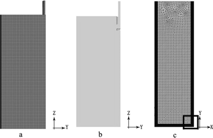
A schematic view of the slab domain modeled along with grid distributions (a) mesh of the slab domain (b) A schematic view of the slab domain (c) mesh of slice at 0.8 m from meniscus with surface and edges.

The submerged depth of the SEN is 0.2 m, measured vertically from the meniscus to the middle of the SEN port which is shown in Fig. 1 at the section b. The SEN’s diameter is 0.085 m. And the SEN port is rectangular, with a height of 0.075 m, width of 0.07 m and 15 degree downwards.

3.1. Inclusion Capturing

3.1.1. Inclusion Capturing Condition

Inclusions capturing condition is defined by the liquid fraction f, when f<0.2 which means the solid fraction is up 0.8,³³⁾ maximum diameter of inclusions and molten steel velocity when the solid fraction is 0.8 must meet the requirements showed in Fig. 2. The result of this work showed in Fig. 3. As section b of the figure shows that the maximum velocity of the molten steel is 0.06 m/s when the solid fraction is 0.8. Considering the max size of the inclusion is 195 μm, all size of the inclusions meet the capturing requirement after adding this data to the Fig. 2 if arriving at solid shell which solid fraction is 0.8. Figure 2 shows the work of Miki Yuji³³⁾ and Yamada Wataru’s work³⁴⁾ about the relationship between steel flow velocity and maximum diameter of inclusions when the inclusions can be captured.

Fig. 2.

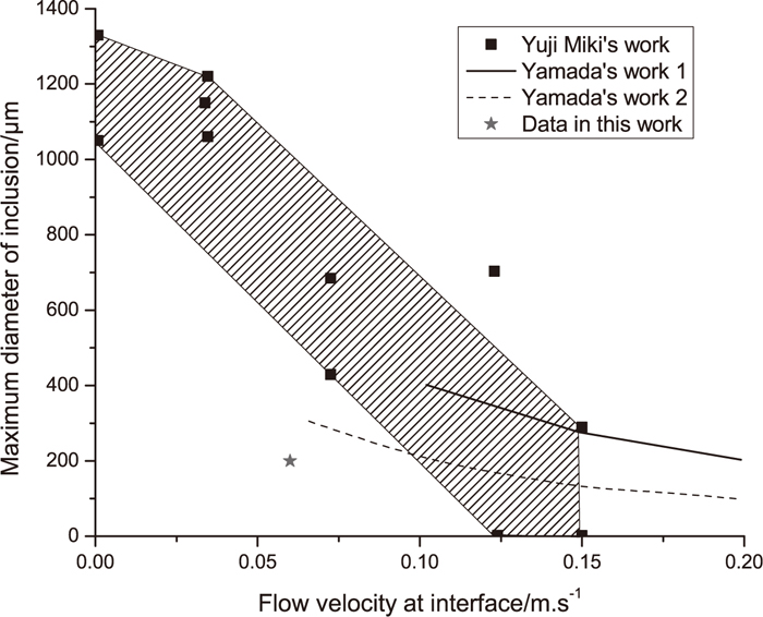
Relationship between steel flow velocity and maximum diameter of inclusions.

Fig. 3.

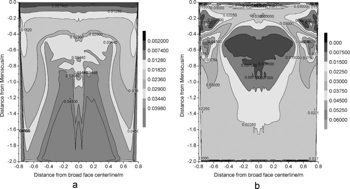
(a) Distribution of shell thickness defined by 0.8 solid fraction (m) (b) Velocity of the molten steel when the solid fraction is 0.8 (m/s).

As the section a of the Fig. 3 shows that the distribution of shell thickness is uneven in the continue casting process when using the 0.8 solid fraction defines the shell thickness. The capturing of the inclusion becomes uneven after considering the uneven distribution of the shell thickness and the velocity of the molten steel when the solid fraction is 0.8.

According to the study of Miki Yuji³³⁾ and Kusuhiro Mukai,²⁶⁾ the forces acting on the inclusion near solid/liquid interface are drawn in Fig. 4. The inclusion is governed by the Saffman force and Suction force caused by the concentration gradient at the same time when the inclusion is in concentration boundary layer, only governed by the Saffman force when the inclusion is between velocity boundary layer and concentration boundary layer and governed by neither when the inclusion beyond the velocity boundary layer.

Fig. 4.

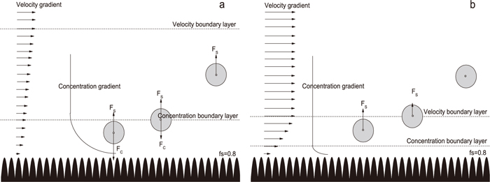
Schematic drawing of steel flow velocity gradient, inclusion concentration gradient and force on particle near solid/liquid interface (no considering buoyant force) (a) small flow velocity near solid/liquid interface (b) large flow velocity near solid/liquid interface.

3.1.2. Result of Simulation

Simulation of inclusion capturing includes flow of the liquid steel, heat transfer of the slab and momentum of the lagrangian discrete phase. In order to study the distribution of the inclusions in the surface layer of the slab, the velocity of the slab and solidification of the slab are discussed in flowing paper.

The distribution of different size inclusion at 5 time point including 10 s, 30 s, 100 s, 200 s, 300 s showed in the Fig. 5 with the quarter model. The area of inclusion distribution become larger and larger with the time showed in Fig. 5. At the same time some large inclusion moves upward with the influence of the buoyant force, and the large number of small inclusions flow with the liquid steel. Lots of the large inclusion float up at 0–30 s, but there are some large inclusion flowing with the liquid steel and mixing with the small inclusions at 30–300 s.

Fig. 5.

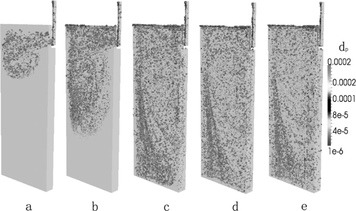
Distribution of inclusions at different time (0–300 s) (a) 10 s (b) 30 s (c) 100 s (d) 200 s (d) 300 s.

After 200 s, the distribution of the inclusions changes very little, because the number of inclusions which injected from the inlet of SEN equal to the ones which escape from outlet and removed by the upper surface.

In order to study the solidification of the surface layer in the slab, slices of different distance from inner surface with the liquid faction are given out in the Fig. 6. With the increasing of distance from inner surface, the uneven distribution of the solidification becomes more and more obvious. Solidification of the middle broad face is faster than the edge ones.

Fig. 6.

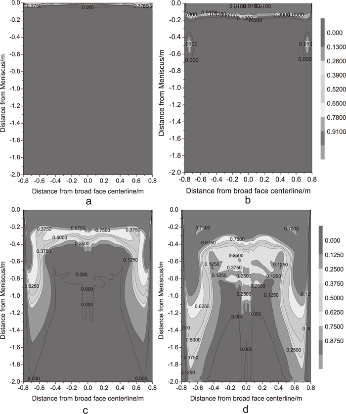
Uneven distribution of solidification with liquid fraction (a) 0.005 m from inner surface (b) 0.015 m from inner surface (c) 0.022 m from inner surface (d) 0.035 m from inner surface.

The distribution of the inclusions at different distance from the inner surface is shown in Fig. 7 with shadow inclusion capturing area and pattern sample area. It is found that the inclusions cluster at the quarter of 0.01–0.03 m from the inner surface in section b, c. But the large inclusions which over 100 μm cluster at 0.00–0.03 m from the inner surface in section a, b, c. The inclusion capturing area is 0.0–0.1 m from meniscus in the section a of Fig. 7, 0.1–0.4 m from meniscus in the section b and uneven distribute in section c and d. The sample area is used for experiment and simulation data analysis.

Fig. 7.

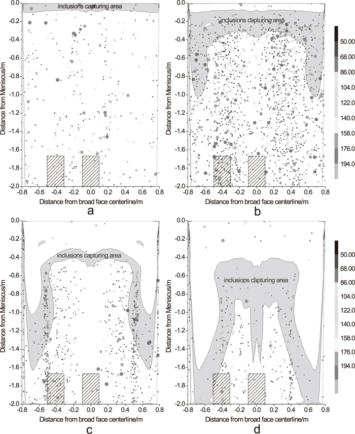
Distribution of inclusions (size in μm) at different slice with capturing area (shadow area) and sample area (pattern area) (a) 0–0.01 m from inner surface (b) 0.01–0.02 m from inner surface (c) 0.02–0.03 m from inner surface (d) 0.03–0.04 m from inner surface.

3.2. Discussion

3.2.1. Experimental Method

The extraction of a metal sample was made by using a potentiometric electrolytic extraction technique with 95% ethanol+FeCl₃ with the device showed in Fig. 8. To avoid oxidation of the steel, argon(Ar) atmosphere was used. The amount of dissolved metal was about 80 g–120 g, the sample section is the pattern area showed in Fig. 7, and the sample is 0.1 m wide, 0.15 m long and 0.01 m thick. The electrolyte solution was filtered by using nylon membrane filter of an open pore size of 50 μm. Then the inclusions are weighed by a balance which is one ten-thousandth part of one gram precision. The particles size were measured by stereoscope at a magnification of 30–45. The size and the chemical composition of particles were analyzed by SEM and EDS.

Fig. 8.

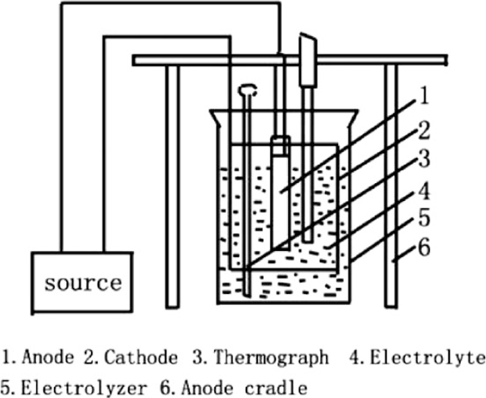
Schematic view diagram of Electrolytic device.

The inclusion content on the quarter of the broad face has a maximum value at 0.02–0.03 m below the surface, and the inclusion content on the half of the broad face has a maximum value at 0.01–0.02 m below the surface shown in Fig. 9. At the same time the total inclusion content on the quarter of the broad face at each distance from the inner arc surface is more than the center one.

Fig. 9.

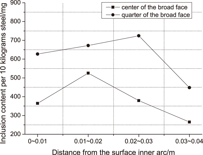
Inclusion content at the broad face varies with the distance from the inner surface (inclusion size over 50 μm).

3.2.2. Comparison Simulation with Experiment

The simulation data is obtained by cutting the sample data block from the sample section showed in Fig. 7, calculate the weight of the inclusion by equation ${\text{m}}_{\text{p}}={\sum }_{\text{i}=0}^{\text{n}}\frac{4}{3}\pi {\text{r}}_{\text{p},\text{i}}^3{\rho }_{\text{p}}$ , where n is the max number of the inclusion in 1, ρ_p is the density of the inclusion in kg/m³, r_{p, i} is the i-th radius of the inclusion. Then the following figures are given out.

Comparison of the inclusion mass percentage at the quarter of broad face varies the distance from the inner surface by cutting the slice at the pattern area in section a, b, c, d of Fig. 7 which inclusion size over 50 μm is showed in section a of Fig. 10. The inclusion mass distribution of numerical simulation is similar to experiment one. The inclusions cluster at the quarter of 0.01–0.03 m from the inner surface which has also been observed in Fig. 7.

Fig. 10.

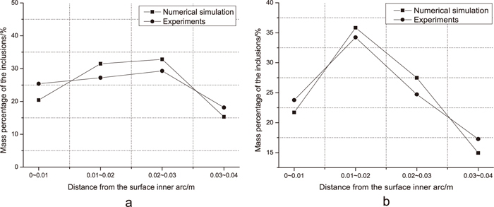
Comparison of inclusion mass percentage varies with the distance from the inner surface (inclusion size over 50 μm) (a) at the quarter of broad face (b) at the center of broad face.

The experiment data of section b in Fig. 10 shows that the inclusion cluster at the center of 0.01–0.02 m from the inner surface, and the numerical simulation one also shows that the inclusions cluster at the quarter of 0.01–0.02 m from the inner surface. The distribution of the inclusions is similar in the two cases.

Comparison of the inclusion total mass percentage at different position of broad face is showed in Fig. 11. The data shows that the inclusions cluster at the quarter of broad face. The numerical simulation data is similar to the experiment ones.

Fig. 11.

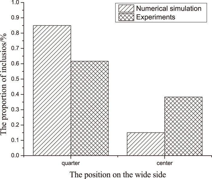
Comparison of inclusion total mass percentage at different position of broad face (inclusion size over 50 μm).

4. Conclusions

This work investigated inclusion motion phenomena during the solidification process of casting slab. Inclusion distribution, inclusion trajectories of different distance from inner surface are given in this paper based on the three-dimensional numerical simulation. The solidification front captured the inclusions during the solidification process of casting slab are showed in this paper and the comparison of the experiment data with the simulation one is given out.

Most of the large inclusions float up at 0–30 s, but the other flow with the liquid steel and mix with the small ones. With the solidification front capturing and the influence of the flow stream, the distribution of the inclusion in the inner surface layer becomes uneven. Most of the inclusions cluster at the quarter of the broad face, and large inclusions cluster at 0.01–0.03 m from the inner surface, small inclusions cluster at 0.02–0.04 m from the inner surface.

The proportion of inclusion shows that the inclusions cluster at the quarter of broad face by comparing the quarter data with the center data of the broad face. And the model in this paper can be used to predict the distribution of the inclusions which size is over 50 μm in the surface layer of the slab for the simulation data agree well with the experiment data.

Acknowledgements

The authors gratefully express their appreciation to National Natural Science Fund of China (51174024) for sponsoring this work.

Nomenclature

A_mush: Mushy zone constant

C_1ε, C_2ε, C_μ: Turbulent constant

C_D: Dimensionless drag coefficient as a function of particle

C_L: Solute concentration in the boundary layer

C₀: Solute concentration in molten steel

c_p: Specific heat at constant pressure

D_L: Diffusion coefficient of solute

d_p: Particle diameter

e: Small number (0.001)

ε: Turbulence kinetic energy rate

f: Liquid volume fraction

F_c: Suction force caused by the concentration gradient

F_drag: Drag force per unit particle mass

F_i: Additional force per unit particle mass

F_s: Saffman force

G_K: Generation of turbulence kinetic energy due to the mean velocity gradients

h: Sensible enthalpy

H: Enthalpy

ΔH: Latent heat

H_latentHeat: Special latent heat

h_ref: Reference enthalpy

k: Thermal conductivity

K: Turbulent kinetic energy

K_c: Gradient of interfacial tension in the boundary layer

K_eff: Effective thermal conductivity

K_E: Effective distribution coefficient

k_t: Turbulent thermal conductivity

K₀: Equilibrium distribution coefficient

p: Static pressure

ρ: Density of molten steel

ρ_p: Density of the particle

R: Radius of the particle

Re_p: Particle Reynolds number

S_U: Momentum source

T_liquidus: Liquidus temperature

T_ref: Reference temperature

T_solidus: Solidus temperature

U: Velocity of the fluid steel

U_cast: Casting speed

U_p: Particle velocity

$\overline{\mathrm{U}}$ : Mean fluid phase velocity

U′: Gaussion distributed random velocity fluctuation

μ: Viscosity of the fluid steel

μ_eff: Effective viscosity of the fluid steel

μ_t: Turbulent viscosity

ν: Kinematic viscosity of the liquid steel

V_s: Moving speed of the solidification interface

δ: Thickness of concentration boundary layer

σ: Interfacial tension of the inclusions in the molten steel

σ_K, σ_ε: Turbulent constant

References

• 1)   S. H.  Seyedein and  M.  Hasan: Int. J. Heat Mass Tran., 18 (1997), 4405.
• 2)   S. K.  Choudhary and  D.  Mazumdar: ISIJ Int., 7 (1994), 584.
• 3)   X.  Huang,  B. G.  Thomas and  F. M.  Najjar: Metall. Mater. Trans. B, 3 (1992), 339.
• 4)   P. J.  Flint: Steelmaking Conf. Proc., ISS, Warrendale, PA, (1990), 481.
• 5)   A. D.  Brent,  V. R.  Voller and  K. T. J.  Reid: Numer. Heat Tr. A-Appl., 3 (1988), 297.
• 6)   H.  Yang,  X.  Zhang,  K.  Deng,  W.  Li,  Y.  Gan and  L.  Zhao: Metall. Mater. Trans. B, 6 (1998), 1345.
• 7)   Y.  Miki,  Y.  Shimada,  B. G.  Thomas and  A.  Denissov: Steelmaking Conf. Proc., ISS, Warrendale, PA, (1997), 37.
• 8)   Y.  Miki and  B.G.  Thomas: Metall. Mater. Trans. B, 4 (1999), 639.
• 9)   S.  Lopez-Ramirez,  J.  Palafox-Ramos,  R. D.  Morales,  J. D. J.  Barreto and  D.  Zacharias: Metall. Mater. Trans. B, 4 (2001), 615.
• 10)   S.  Joo,  J.W.  Han and  R.  Guthrie: Metall. Mater. Trans. B, 5 (1993), 767.
• 11)   K.  Takatani,  Y.  Shirota,  Y.  Higuchi and  Y.  Tanizawa: Model. Simul. Mater. Sci., 3 (1999), 265.
• 12)   H.  Lei,  M. Y.  Zhu and  J. C.  He: Guocheng Gongcheng Xuebao (Chinese J. Process Eng.), (China), 2 (2001), 138.
• 13)   L.  Zhang,  Y.  Wang and  X.  Zuo: Metall. Mater. Trans. B, 4 (2008), 534.
• 14)   M. D.  Santis and  A.  Ferretti: ISIJ Int., 6 (1996), 673.
• 15)   M. R.  Aboutalebi,  M.  Hasan and  R. I. L.  Guthrie: Metall. Mater. Trans. B, 4 (1995), 731.
• 16)   H.  Lei,  D. Q.  Geng and  J. C.  He: ISIJ Int., 10 (2009), 1575.
• 17)   L.  Zhang,  J.  Aoki and  B. G.  Thomas: Metall. Mater. Trans. B, 3 (2006), 361.
• 18)   L. T.  Wang,  Q. Y.  Zhang,  S. H.  Peng and  Z. B.  Li: ISIJ Int., 3 (2005), 331.
• 19)   R. B.  Bird,  W. E.  Stewart and  E. N.  Lightfoot: Transport Phenomena, ed. by R. B. Bird, W. E. Stewart and E. N. Lightfoot, Wiley, New York, (2006).
• 20)   T.  Shih,  W. W.  Liou,  A.  Shabbir,  Z.  Yang and  J.  Zhu: Comput. Fluid., 3 (1995), 227.
• 21)   B. A.  Kader: Int. J. Heat Mass Tran., 24 (1981), 1541.
• 22)   B. E.  Launder and  D. B.  Spalding: Comput. Method. Appl. M., 2 (1974), 269.
• 23)   P.  Saffman: J. Fluid Mech., 2 (1965), 385.
• 24)   K.  Mukai and  W.  Lin: Tetsu-to-Hagané, 7 (1994), 533.
• 25)   J. D.  Schwarzkopf,  M.  Sommerfeld and  Y.  Tsuji: Multiphase Flows with Droplets and Particles, ed. by J. D. Schwarzkopf, M. Sommerfeld and Y. Tsuji, CRC Press, Boca Raton, Florida, (2011).
• 26)   K.  Mukai and  W.  Lin: Tetsu-to-Hagané, 7 (1994), 527.
• 27)   M. C.  Flemings: Solidification Processing, ed. by M. C. Flemings, McGraw-Hill College, New York, (1974).
• 28)   L. L.  Baxter and  P. J.  Smith: Energ. Fuel., 6 (1993), 852.
• 29)   K.  Lai,  M.  Salcudean,  S.  Tanaka and  R.  Guthrie: Metall. Mater. Trans. B, 3 (1986), 449.
• 30)   C.  Offerman: Scand. J. Metall., (1981), 25.
• 31)   S. H.  Seyedein and  M.  Hasan: Int. J. Heat Mass Tran., 18 (1997), 4405.
• 32)   R.  Davies,  N.  Blake and  P.  Campbell: 4 th Int. Conf. Continuous Casting, Preprints, Düsseldorf, FRG, Brussels, Belgium, (1988), 645.
• 33)   Y.  Miki,  H.  Ohno,  Y.  Kishimoto and  S.  Tanaka: Tetsu-to-Hagané, 8 (2011), 423.
• 34)   W.  Yamada,  A.  Kiyose,  J.  Nakajima,  A.  Fukuda,  K.  Okazawa and  K.  Miyazawa: CAMP-ISIJ, 12 (1999), 682.
• 35)   X.  Huang and  B. G.  Thomas: Can. Metall. Q., 3-4 (1998), 197.