Optimization of Combined Blown Converter Process

Abstract

A 1/6th scaled down physical model was used to study and optimize the stirring condition of a 30 t converter. A number of parameters were studied and their effects on the mixing time were recorded. A new bottom tuyere scheme with an asymmetrical configuration was found to be one of the best cases with respect to a decreased mixing time in the bath. Mathematical modeling was employed to study the flow field characteristics caused by the new tuyere scheme. In the mathematical model, a comparison between the existing and the new tuyere setups was made with regards to the mixing time and turbulence in the bath. In addition, a new volumetric method for calculating the mixing time was applied. The results showed that, on average, a 23.1% longer mixing time resulted from the volumetric method compared to the standard method where discrete point are used to track the mixing time. Furthermore, an industrial investigation was performed to check the effects of the new tuyere scheme in a converter by analyzing the [O], [C] and [P] contents in the bath. The results showed that the application effects of the new tuyere scheme yield a better stirring condition in the bath compared to the original case.

1. Introduction

Today, the top and bottom combined blown converter is commonly used in primary steel making plants. In the combined converter, the agitating and the mixing of the bath are forced by the top oxygen jets and the bottom gas plumes, which can achieve a high mixing efficiency for the bath. The top-lance height, the gas flow rates, side blowing and bottom blowing are investigated parameters used to improve the steel making process in many studies. Evidently, the bottom tuyere configuration in the combined blown converter is very significant to the bath mixing, reaction of slag-metal and splashing. Vikas et al.¹⁾ carried out a water model study of a combined blown converter in order to optimize the locations of the bottom blowing nozzles with respect to the mixing time. A mathematical model was also used to simulate the bottom blowing in the converter. Overall, the computational results showed a good agreement with that of the experimental observations in some of the cases. Shiv et al.²⁾ used a cold model and thermodynamic analysis to evaluate the bottom stirring of the system, they found that the dolomite lining life of the vessel increases and the total Fe content of the slag decreases with an increased bottom stirring.

There are few reports^3,4,5) on combined blowing in mathematical simulation. Wei et al.^3,4) developed a mathematical model of a side and a top combined blown AOD converter. The changes and the number of the tuyere in the AOD were investigated. The results showed that the fluid flow in the bath can be reliably predicted. In the research of Odenthal et al.⁵⁾ research, a combined VOF and DPM model was used to describe the 3D, transient and non-isothermal flow of the melt, slag, and oxygen for a 335 t combined blown converter.

In the current study, the optimized approach of the bottom-tuyere configuration has been described in previous work;⁶⁾ the distribution of the bottom tuyeres was optimized based on experimental findings from the physical top and bottom combined blown converter model. Then, the mathematical models were built to describe the fluid flow characteristics in the bath of the original and the optimized tuyere schemes. A new calculation method for mixing time of the bath was applied in this study. The whole region of the bath can be considered in the change of the tracer concentration to avoid the defects brought by the discrete-point method. Moreover, to further verify the impact of the new tuyere setup, an industrial investigation was carried out to study the differences in species concentrations between the original scheme and the optimized scheme at tapping.

2. Physical Model

The physical model was scaled down in a 1:6 ratio of the industrial 30 t combined blown converter. The experiments were carried out with the experimental apparatus shown in Fig. 1. Water and compressed air were used to simulate the liquid steel and oxygen in the bath, respectively. The modified Froude number Fr′ (Eq. (1)) was applied to select the appropriate conditions (Table 1) for both bottom- and top- blowing gas.   

$$Fr\prime =\frac{{\rho }_l}{{\rho }_l-{\rho }_g}\cdot \frac{v^2}{gH}$$(1)

where

ρ_l is water density,

ρ_g is air density,

v is the velocity of gas,

g is the acceleration of gravity,

H is the diameter of tuyeres and nozzle.

Fig. 1.

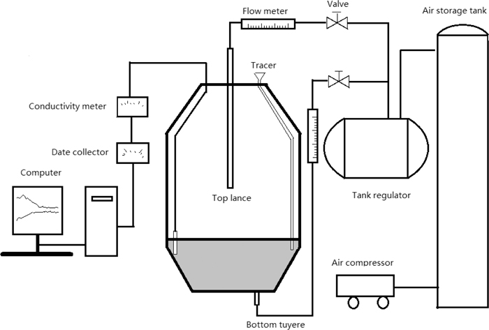
Schematic illustration of the experimental setup.

Table 1. The parameters in the experiment.

Parameter	Prototype	Physical model
Diameter of the vessel, mm	2950/2500	492/417
Height of the bath, mm	900	150
Height of the lance, mm	800, 950, 1100	133, 158, 183
Number of bottom tuyeres	3	3
Top gas flow rate, Nm3/h	7600	34.66
Bottom gas flow rate, Nm3/h	50, 90, 180, 270	0.21, 0.47, 0.94, 1.21

To optimize the combined blown converter, a number of bottom-tuyere configurations were tested in order to optimize the dynamic conditions of the bath. Several schemes were found to be effective in improving the mixing effects. The bottom blown converter was also studied to find an appropriate flow rate of blowing gas. In addition, the influence of different top-lance heights were investigated since the top-lance height is adjusted in real practice.

In this paper, an optimized scheme with bottom-tuyere configured asymmetrically was chosen to show the optimized results and it was also used as the reference scheme of the mathematical simulation. Figure 2 shows the distribution of bottom tuyeres in the original and the optimized scheme. To eliminate other influencing factors, the top blowing gas flow rate was kept constant in both cases. In the physical experiment, a mean value of the mixing times measured from 3 different probes was determined and regarded as the bath mixing time. In the physical model, mixing time is the time measured starting from the instant of the tracer addition to the point where the tracer concentration reaches 99% of the homogeneous value.

Fig. 2.

The bottom tuyere distribution of the converter. The three blowing directions of the top lance can also be seen in the figure.

3. Mathematical Model

A combination of a volume of fluid (VOF) and a discrete phase model (DPM) were used in order to describe the combined blown in the converter model. The UDS (user defined scalar) model was performed to calculate the mixing time in the bath of the converter.⁷⁾

3.1. VOF Model

A coupled level-set and VOF model⁸⁾ was used in the simulation. The level-set method is used for producing accurate estimates of interface curvature and surface tension force. The tracking of the interface between air and liquid is accomplished by the solution of a continuity equation for the volume of air or liquid phase. For the q^th phase, the equation has the following form:⁷⁾   

$$\frac{\partial {\alpha }_q{\rho }_q}{\partial t}+\overrightarrow{\nu }\cdot \nabla {\alpha }_q{\rho }_q=0$$(2)

The primary-phase volume fraction is computed based on the following constraint:   

$${\sum }_{q=1}^n{\alpha }_q=1$$(3)

The momentum equation, shown as below, is dependent on the volume fractions of the air and the water phases through the properties ρ and μ:   

$$\frac{\partial }{\partial t}\left(\rho \overrightarrow{v}\right)+\nabla \left(\rho \overrightarrow{v}\overrightarrow{v}\right)=-\nabla p+\nabla \cdot \left[\mu \left(\nabla \overrightarrow{v}+\nabla {\overrightarrow{v}}^T\right)\right]+\rho \overrightarrow{g}+\overrightarrow{F}$$(4)

where

p is the static pressure,

ρ_g is the gravitational force,

F is the external body force and model-dependent source terms,

ρ and μ are shown as below:   

$$\rho ={\rho }_{\text{air}}{\alpha }_{\text{air}}+\left(1-{\alpha }_{\text{air}}\right){\rho }_{\text{liquid}}$$(5)

  

$$\mu ={\mu }_{\text{air}}{\alpha }_{\text{air}}+\left(1-{\alpha }_{\text{air}}\right){\mu }_{\text{liquid}}$$(6)

3.2. DPM Model⁷⁾

The water in the simulation was treated as a continuous phase by solving the Navier-Stokes equations, while the bubbles used in the bottom blowing were described by the discrete phase model. A user defined function (UDF) was used to delete the discrete phase bubbles when they reached the liquid/gas interphase. Thus, it was assumed that the bubbles would escape to the gas above the interphase in this case.

The trajectory of the bubbles was predicted by integrating the force balance on the bubbles. This force balance equates the bubbles inertia with the forces acting on the bubbles, and can be shown as follows:   

$$\frac{d{v}_b}{dt}=F_D\left(\overrightarrow{v}-\overrightarrow{v_b}\right)+\frac{\overrightarrow{g}\left({\rho }_b-\rho \right)}{{\rho }_b}+\overrightarrow{F}$$(7)

where

v is the water velocity in the bath,

v_b is the velocity of the bubbles,

ρ_b is the density of bubble,

ρ is the density of water,

F is an additional acceleration term,

${\text{F}}_{\text{D}}\left(\overrightarrow{\mathrm{v}}-\overrightarrow{{\mathrm{v}}_{\mathrm{b}}}\right)$ is the drag force per unit bubble mass and   

$$F_D=\frac{18\mu }{{\rho }_b{d}_b^2}\frac{C_{D}Re}{24}$$(8)

here, μ is the molecular viscosity of the water; C_D is the drag coefficient of the bubbles.

Another UDF for the discrete phase model was used to describe the drag force of bubbles in the water. The shape of bottom blown bubbles is irregular in the bath, especially when the diameters of the bubbles are large and the flow rate is high. As a result, the rigid sphere drag force coefficient is not suitable to describe all the bubbles mathematically. Ellipsoidal shape and cap shape bubbles are in majority in the experiments and the bubble shape will affect the bubble drag force. Therefore, the water flow in the bath was roughly divided into two turbulent regions based on the Reynolds number. This is due to that the shape of the bubbles in the water is affected by the Reynolds number. The drag force coefficient is defined as follow⁹⁾   

$$C_D=\{\begin{array}{c}\frac{64}{\pi Re}\cdot \left(1+0.138{\text{Re}}^{0.792}\right),\hspace{1em}\left(Re\le 133\right)\\ \hspace{1em}\hspace{1em}\hspace{1em}\hspace{1em}\hspace{1em}\hspace{1em}\mathrm{\hspace{0.17em} }\mathrm{\hspace{0.17em} }1.17,\hspace{1em}\hspace{1em}\hspace{1em}\hspace{1em}\left(Re>133\right)\end{array}$$(9)

Re is the relative Reynolds number, which is define as   

$$Re\equiv \frac{\rho d_b\left|\overrightarrow{v}-\overrightarrow{v_b}\right|}{\mu }$$(10)

where

ρ is the density of water,

d_b is the bubble diameter,

v is the velocity of the water,

v_b the velocity of the bubbles,

μ is the molecular viscosity of the water.

The additional acceleration F includes the “virtual mass” force^7,10) and the “pressure gradient” force⁷⁾ and can be written as Eqs. (11) and (12), respectively.   

$$F_{virtual}=\frac{1}{2}\frac{\rho }{{\rho }_b}\frac{d}{dt}\left(\overrightarrow{v}-\overrightarrow{v_b}\right)$$(11)

  

$$F_{pressure}=\frac{\rho }{{\rho }_b}{v}_b\nabla v$$(12)

In the DPM model, the node-based averaging method⁷⁾ was applied to distribute the bubble’s effects to neighbouring mesh nodes. The grid dependency of bubbles simulation can be reduced since the bubbles effects on the flow solver are distribute more smoothly across neighbouring cells.

3.3. Turbulence Equations

The Standard k-ε model¹¹⁾ was used to describe turbulence, which solves equations to obtain the eddy viscosity field:   

$${\mu }_t=\rho C_{\mu }{k}^2/\epsilon$$(13)

For the standard k-ε model, the turbulence kinetic energy, k, and its rate of dissipation, ε, are calculated from the following transport equations:   

$$\frac{\partial }{\partial t}\left(\rho k\right)+\frac{\partial }{\partial x_i}\left(\rho u_{i}k\right)=\frac{\partial }{\partial x_j}\left(\left(\mu +\frac{{\mu }_t}{{\mathrm{\sigma }}_k}\right)\frac{\partial k}{\partial x_j}\right)+G_k-\rho \epsilon$$(14)

and   

$$\begin{array}{l}\frac{\partial }{\partial t}\left(\rho \epsilon \right)+\frac{\partial }{\partial x_i}\left(\rho u_i\epsilon \right)=\frac{\partial }{\partial x_j}\left(\left(\mu +\frac{{\mu }_t}{{\mathrm{\sigma }}_{\epsilon }}\right)\frac{\partial \epsilon }{\partial x_j}\right)\\ +G_{1\epsilon }\left(G_k+G_{3\epsilon }{G}_b\right)\frac{\epsilon }{k}-G_{2\epsilon }\frac{{\epsilon }^2}{k}\rho \end{array}$$(15)

in the equations, G_k represents the generation of turbulence kinetic energy due to the mean velocity gradient, calculated as described as follows:   

$$G_k={\mu }_i\frac{\partial u_j}{\partial x_i}\left(\frac{\partial u_i}{\partial x_j}+\frac{\partial u_j}{\partial x_i}\right)$$(16)

where C₁ε, C₂ε, σ_k, σ_ε and C_μ are constant and have the following default values,¹¹⁾ C_1ε=1.44, C_2ε=1.92, C_μ=0.09, σ_k=1.0, σ_ε=1.3.

3.4. User-Defined Scalar

The mixing time of the bath is the main parameter used to study the stirring effects in both the physical model and the mathematical model. The simulation of the mixing time uses a User-Defined Scalar model, which solves the following equation:⁷⁾   

$$\frac{\partial }{\partial t}\left(\rho \varnothing \right)+\frac{\partial }{\partial x_i}\left(\rho u_i\varnothing -\mathrm{\Gamma }\frac{\partial \varphi }{\partial x_i}\right)=0$$(17)

where Γ is the diffusion coefficient in turbulent flows, which is computed in the following form:   

$$\mathrm{\Gamma }=\rho D_m+\frac{{\mu }_t}{S{C}_t}$$(18)

here, D_m is the mass diffusion coefficient , SC_t is the turbulent Schmidt number (μ_t /ρD_t where μ_t is the turbulent viscosity and D_t is the turbulent diffusivity).

3.5. Boundary Conditions and Solution Methods

A velocity boundary profile was set as the top-inlet boundary condition according to the methodology described in a previous paper.¹²⁾ Different mass flow rates inlet boundary conditions of bottom-blowing gas were used with the DPM model. A pressure outlet boundary condition was employed for the outlet of the converter model in this case. The relative static pressure at the outlet boundary was assumed to be at atmosphere pressure and was set to zero. A standard wall function was selected to model the velocity near the wall and a no-slip wall condition was used at the wall.

A Cutcell⁷⁾ 3D grid was developed to represent the computational domain. A fine mesh at the liquid/gas interface and high velocity-gradient regions together with the Geo-reconstruct algorithm were used to track the free surface deformation due to top- and bottom- blowing. Pressure-velocity coupling was solved using the PISO algorithm.⁷⁾ The second upwind scheme was chosen for momentum and turbulence in the spatial discretization. The time steps used in the fluid simulations were 0.2 ms. However, for mixing time calculations a frozen flow field was used. In this case, the time-step could be increased to 10 ms in those simulations. The simulations were run long enough time for a fully developed flow to develop. This flow field was acquired by monitoring the velocity of the fluid in the bath. The calculation results were saved every 5 seconds to enable a calculation of the mixing times by using the frozen flow fields.

The comparisons of penetration depth of top blowing has been done between coarse (54093), medium (101721) and fine (258730) mesh in order to test the mesh sensitivity. The cavity depth calculated with coarse mesh is 0.021 m, which has 46% difference with the result (0.039 m) in medium mesh calculation. The variation between calculated with medium and fine mesh is decreased by less than 2.5%. Because it takes a long time to get the solution with fine mesh, the medium mesh was applied in this study. During the calculation, the grid was varied from 100000 to 150000 with the mesh refined in the region where the velocity and phase gradient is high.

The mathematical model was built using the commercial CFD software ANSYS^® 14.5 and the calculations were carried out on a Win7 PC with 3.19 GHz Intel Core i7 CPU. Normally, 24 hours were needed to complete a 5 seconds long simulation and more than 1 month for a simulation of a complete case.

4. Industrial Experiments

To verify the new tuyere configuration found using of the physical and the mathematical models, some industrial experiments were performed in a 30 t combined converter. The study method in the industrial experiment was a bit different from that of the physical and the mathematical models due to the high temperature, which makes the mixing effects of the bath difficult to measure directly. However, the flow field, which is affected by the gas flow rates, can partly be reflected by the C, O and P content in the liquid steel. As a result, the original and the optimized converter experiment results were compared by studying the content of these elements in the liquid steel at tapping. Table 2 shows the raw material and gas supply in the experiment.

Table 2. The industrial experiment conditions.

	Parameter
Hot metal, t	23–25	C/wt%	4.0–4.5
		P/wt%	0.067–0.138
		T/°C	1271–1312
Scrap, t	3–4
Pig iron, t	5–6
Top gas oxygen flow rate, Nm3/h	7600–7800
Top-lance height, m	0.8–1.2
Bottom gas flow rate, Nm3/h	0.046–0.05

The experiments were set up in such a way as to minimize the differences in composition and temperature between each heat, so that only the effects of the stirring could be investigated in spite of the elements’ content in the hot metal, as well as the mass of raw material and gas, is not a constant value in the industrial experiments.

5. Results and Discussion

5.1. Physical Model Results

The mixing times at elevated gas flow rates for the bath are indicated in Fig. 3. Generally, the mixing time decreases with an increased bottom gas flow rate, as can be seen from the figure. However, several inverse trends are also achieved in the experiments. Some critical flow rates are also observed from the experimental results in which an extra gas supply lead to unobvious changes or opposite effects in mixing time. This indicates that higher bottom flow rates of bottom blown may not always give positive effects to the stirring of the bath. As shown in Fig. 3, the mixing time increases with increasing bottom flow rates that are higher than 0.47 Nm³/h, when the original scheme is employed with a 158 mm top-lance height. Some similar tendencies can be found when a 133 mm lance height was used in both the original and the optimized schemes.

Fig. 3.

Mixing time in the combined blown converter versus the flow rates from the bottom tuyeres.

It may be seen that a lower top-lance height shows significantly shorter mixing times than that of the higher one for both the original and the optimized schemes. This indicates that a lower top-lance height is better for the mixing effects in the bath, at least for the current span of flow rates. However, the collision between top jets and bottom plume on the surface of the bath shall also be considered more during the change of the lance height.

The mixing times with the optimized scheme are shorter than those of the original scheme for all the top-lance heights and corresponding bottom blowing rates. This means that the optimized scheme of the converter is better in stirring the bath than that of the original one. The mixing times have been decreased by 13.6%, 21.2% and 27.1% for top-lance heights of 133 mm, 158 mm and 183 mm at a bottom blowing rate of 0.47 Nm³/h, respectively. Therefore, it is reasonable to believe that better stirring effects can be achieved in practice when the height of the top lance is adjusted during the process.

In the plant, the bottom blowing rates are from 50 Nm³/h to 270 Nm³/h, which corresponds to 0.21 Nm³/h to 1.21 Nm³/h in the experiment. According to the experimental results, a bottom blowing rate above 0.94 Nm³/h (180 Nm³/h in the plant) is not recommended.

5.2. Mathematical Model Results

As presented in the physical model, too high bottom blowing rates may give negative results and are not recommended to use in plants. Therefore, to make the simulations representative, a blowing rate of 0.47 Nm³/h and a 158 mm top-lance height are chosen as a reference in both the original scheme and the optimized scheme.

To investigate the flow field of the bath in this study, a fully-developed flow is required for performing the mixing-time calculation. Consequently, a velocity-monitor method was applied to monitor the flow velocity in the bath to estimate the flow condition during the calculation process. Figure 4 shows a velocity-monitor result in the combined blown calculation. It can be seen that the calculation region can be divided into two regions. These are roughly separated by a critical value of 65 s roughly by considering the velocity fluctuation and changing tendency. With a low value at the beginning in the monitor point, the velocity as well as the fluctuating intensity in the non-developed region increases. Approximately, the flow field after 65 s is seen as a fully developed flow although it is still an unsteady state flow with high fluctuations. The flow fields are chosen from this fully developed region to investigate the mixing times.

Fig. 4.

The velocity change in the monitor point.

The stirring effects of the bath were investigated by calculating the mixing time of the bath at different simulation times where the flow field is considered to be a developed flow. Five points in time were chosen from the fully-developed flow both in the original and the optimized schemes; the mixing times are shown in Fig. 5. As can be seen from the figure, the total mixing times over the selecting time points revealed a general trend of fluctuations. The bath of the original scheme is in the range of mixing time from 54.1 s to 64.2 s, where the mean value is 59.6 s. For the mixing time in the optimized scheme, it varies between 49.0 s and 55.0 s, with a mean value of 52.0 s. It is clear that the mixing time is decreased by 12.8% in the optimized bath comparing with the original scheme. Note that the mathematical results are slightly higher than those of the physical model in which the corresponding mixing times are 54.3 s and 47.8 s, respectively,

Fig. 5.

The mixing times in the original and the optimized scheme for different blowing times.

The turbulence in the bath is very important to the mixing of the bath. Therefore, the total turbulent kinetic energy of the water in the bath has been checked when the flow is developed. As shown in Fig. 6, fluctuation of turbulent kinetic energy happened both in the original and the optimized bath schemes. However, the fluctuation in the optimized bath gave a higher mean value of 0.14 m²/s², which is 7.4% higher than that of 0.13 m²/s² in the original bath. This indicates that the rearrangement of the bottom tuyeres in the bath changes the turbulence of the bath, as well as the mixing conditions.

Fig. 6.

Comparison of variation of turbulent kinetic energy with time in the bath.

As we know that there are some zones in which the flow field is not active enough with respect to the stirring or some metallurgical vessels where it hard to obtain a suitable stirring; we call this kind of zone is a “dead zone”. However, this kind of zone is very difficult to realize and to locate since the situation can be changed with operating parameters, size of vessels, etc. In this physical model, three probes were used to measure the concentration change of the tracer. But it is very difficult to measure the concentration in the dead zone because too many probes may affect the flow field in the bath. Furthermore, sometimes it is impossible to confirm the location of the dead zone. Therefore, the measured results using probes usually contain a lack of information in the dead zone. Fortunately, numerical tools give investigators chances to consider all regions as the small as mesh size in the studied domain.

The definition of the mixing time using the probe method is similar to that of the physical model. To consider the concentration change of all the regions in the bath, a new mixing time method was applied in this study. The mixing time is calculated based on the volume of 99%–101% homogenization of the scalar over the entire bath volume. Figure 7 shows the differences in the mixing time calculations by different methods. The mixing times based on a discrete point monitor in Fig. 6(a) are 38.7 s, 54.5 s, and 61.5 s, with a mean value of 51.6 s. By considering the whole region of the bath, it took 62.0 s, which is 20.1% longer than that of the discrete point monitor result, to achieve the same homogenous requirement for the bath.

Fig. 7.

The comparison of different mixing time calculations.

As a consequence, the volumetric monitor method was used in the optimized case to calculate the mixing time in the chosen time-point; the results are shown in Fig. 8. Noticeably, all the results calculated by the volumetric method revealed a trend of higher mixing time than those of the discrete point monitor method. This means that some regions in the bath may not reach homogeneousness when the measured points get homogeneous. The differences between the two methods vary from a minimum value of 12.7% to a maximum value of 44.9%, which indicates that the location of the point monitor may greatly affect the results in the calculation. The mean value of mixing time in the volumetric calculation is 64.0 s, which is 23.1% higher than the mean value of 52.0 s determined by the discrete point method. This suggests that the mixing time acquired from the discrete point method is representative to a certain extent. However, the volumetric method should be executed in the mixing time calculation if the dead zones in the bath or vessels are of concern.

Fig. 8.

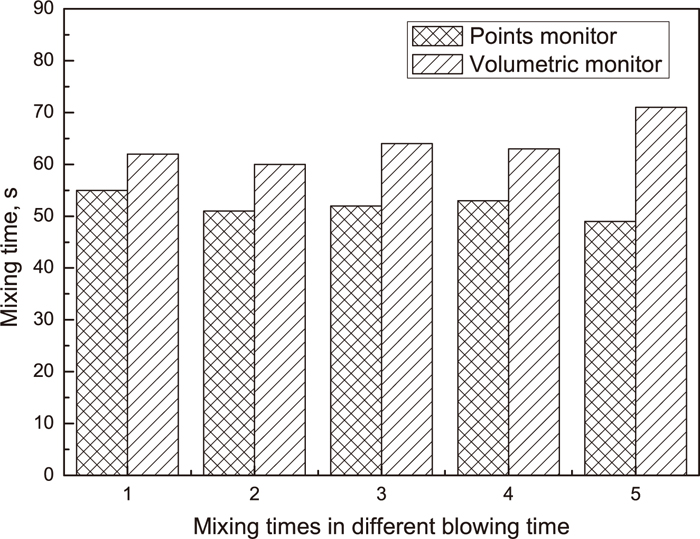
The mixing time differences in different monitor-type.

5.3. Industrial Experimental Results

Figure 9 presents the comparison of C, O and P contents at tapping using both the original and the optimized schemes. As can be seen from the statistics, the O content fluctuates sharply between 0.05% and 0.09% in both the original and the optimized schemes. The O content in the optimized schemes is decreased but sometimes higher in the optimized scheme than that of the original scheme. As a whole, the O content is decreased by 6.0% from 0.067% (original scheme) to 0.063% (optimized scheme) by considering the mean values of all heats in the experiment. However, an obvious C content change has not been found from the results. There is not a great difference between the original and the optimized schemes in C content, which are 0.051% and 0.048%, respectively.

Fig. 9.

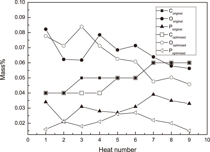
Industrial experiments comparing the original tuyere scheme to the optimized tuyere scheme.

A low P content is one of the main metallurgical requirements in the steel making process using the BOF for most of the steel grades. This is due to that a high P content of the steel will cause a tempering embrittlement, a low ductility and a low strength. A good stirring of the bath can enhance the removing rate of P during the process of the dephosphorization. Since the dephosphorization process occurs between slag and molten steel. An active interface between the slag and the steel is favorable. Consequently, a good stirring with a short mixing time is expected to improve the interaction between the slag and molten steel. Furthermore, the high rates of turbulent diffusion of Phosphorus, which is developed during the vigorous stirring of the bath, can further give a positive effect to the dephosphorization of the steel.

However, dephosphorization is not only affected by stirring energy but also by the composition of the slag and the molten steel as well as the temperature. The experiments were set up in such a way as to minimize the differences in composition and temperature between each heat, so that only the effects of the stirring could be investigated. The samples were taken at tapping and as such it was not possible to see any variation of the Phosphorous content during the process. It is clear that there is an effect due to stirring on the Phosphorous removal.

With the original scheme, the P content is relatively high with a mean value of 0.031%. A favorable result of the optimized scheme can be seen where the P content is significantly decreased; it is 33% lower than for the original scheme. The results from the experiments indicate that the BOF has been optimized successfully and that the stirring effect of the optimized scheme gives a favorable result in practice based on the analyses of elements content at tapping.

6. Conclusions

A new (optimized) tuyere scheme in a combined blown converter is achieved using physical modelling and is evaluated using mathematical modelling as well as industrial experiments. Comparing to the original scheme, which has poor stirring effects to the bath, the new scheme performs favourably with respect to the bath stirring. The specific findings from this study may be summarized as follows:

(1) In the optimized scheme, the mixing times have been decreased 13.6%, 21.2% and 27.1% using top-lance heights of 133 mm, 158 mm and 183 mm and at bottom blowing rate of 0.47 Nm³/h, respectively.

(2) A velocity-monitor method was used to reach a fully-developed flow in the converter bath. The calculated mixing time is decreased by 12.8% in the optimized bath compared to an original stirring scheme. However, the simulation results are slightly higher than that of physical model.

(3) The turbulent kinetic energy in the bath was 7.4% higher in the optimized scheme compared to the original scheme.

(4) A new type of mixing time calculation was employed in the simulations where the entire bath volume was monitored. The volumetric method can calculate concentration changes of the tracer in all the regions of the bath. It revealed a trend of 23.1% higher mixing time than that of the (standard) discrete point mixing time calculations. With an increasing number of discrete point used for the mixing time calculations the two methods should coincide, nevertheless it is important to note that a discrete measurement has a hard time finding all the possible dead zones in a bath. So it is recommended to use the volumetric method, whenever possible, to calculate the mixing time.

(5) Good industrial results were achieved by using the optimized scheme; The C, O and P content were decreased by 5.8%, 6.0% and 33%, respectively. The industrial results are in line with the physical and mathematical modelling which showed a decreased mixing time for the optimized scheme.

Acknowledgment

Xiaobin Zhou would like to extend his sincere grateful to the CSC (China Scholarship Council) for financial support of his PhD study in KTH-Royal Institute of Technology, Sweden.

Nomenclature

α_q : Value of q^th volume fraction [–]

μ : Viscosity [kg·m^–1·s^–1]

μ_t : Turbulent viscosity [kg·m^–1·s^–1]

ρ : Density [kg·m^–3]

ρ_l : Water density [kg·m^–3]

ρ_g : Air density [kg·m^–3]

ε : Turbulence dissipation rate [m²·s^–3]

C : Concentration of tracer in the bath of converter [kg·m^–3]

C₀ : Mean concentration of tracer in the bath of converter [kg·m^–3]

C_D : Drag coefficient of bubbles [–]

D_m : Mass diffusion coefficient [m²·s^–1]

D_t : Turbulent diffusivity [m²·s^–1]

d_b : Diameter of bubbles [m]

Fr’ : Modified Froude number [–]

F : Additional acceleration term [m·s^–2]

F_D : Drag force of bubbles [N]

F_virtual : Virtual mass force [N]

F_pressure : Pressure gradient force [N]

g : Gravitational acceleration [m·s^–2]

H : Characteristic length of tuyere and nozzle [m]

k : Turbulence kinetic energy [m²·s^–2]

p : Static pressure [Pa]

Sc_t : Schmidt number [–]

ν : Velocity of gas [m·s^–1]

ν_b : Velocity of bubbles [m ·s^–1]

ø : Mass fraction for species [–]

Γ : Mass diffusion coefficient for scalar in turbulent flow [m²·s^–1]

References

• 1)   V.  Singh,  J.  Kumar,  C.  Bhanu,  S. K.  Ajmani and  S. K.  Dash: ISIJ Int., 47 (2007), 1605.
• 2)   S. K.  Choudhary and  S. K.  Ajmani: ISIJ Int., 46 (2006), 1171.
• 3)   J. H.  We,  H.  Yuan and  S. G.  Min: Steel Res. Int., 82 (2011), 693.
• 4)   J. H.  Wei,  Y.  Cao,  H. L.  Zhu and  H. B.  Chi: ISIJ Int., 51 (2011), 365.
• 5)   H. J.  Odenthal,  U.  Falkenreck and  J.  Schlüter: European Conf. on Computational Fluid Dynamics, ed. by P. Wesseling et al., TU Delft, The Netherlands, (2006).
• 6)   Z.  Lai,  Z.  Xie and  L.  Zhong: ISIJ Int., 48 (2008), 793.
• 7)  Ansys 14.0 manual, ANSYS, Inc., USA, (2011).
• 8)   C. W.  Hirt and  B. D.  Nichols: J. Comput. Phys., 39 (1984), 201.
• 9)   R.  Clift,  J. R.  Grace and  M. E.  Weber: Bubbles, Drops, and Particles, Academic Press, New York, San Francisco, London, (1978).
• 10)   C. T.  Crowe,  J. D.  Schwarzkopf,  M.  Sommerfeld and  Y.  Tsuji: Multiphase Flows with Droplets and Particles, 2nd ed., CRC Press, USA, (2012), 93.
• 11)   B. E.  Launder and  D. B.  Spalding: Lectures in Mathematical Model of Turbulence, Academic Press, London, England, (1972).
• 12)   X. B.  Zhou,  M.  Ersson,  L. C.  Zhong,  J. K.  Yu and  P.  Jönsson: Steel Res. Int., 85 (2014), 273.