Scheduling Hot Slabs in Parallel Hot Rolling Production Lines by Column Generation

Abstract

This paper is to determine the slab schedule on parallel hot rolling lines with consideration of chain precedence constraints, which restricts the slabs belonging to a chain to be successively processed without interruption in one production line. Moreover, energy loss increases as its waiting time before being processed increases, since the slabs dynamically arrive with high temperature. The objective of the problem is to minimize the total energy loss costs. Two kinds of energy loss cost that are linearly and nonlinearly dependent of its waiting time are concerned. The strongly NP-hard feature of the problem stimulates us to develop branch-and-pricing algorithm to solve it. Firstly, the model is formulated as a set partitioning model. For the strongly NP-hard sub-problem, dynamic programming based on state-space relaxation method is derived to tackle it. A branch-and-bound procedure is applied for the case that the solution obtained at the root node is not integral. The whole algorithm is implemented by C language on a Pentium IV 3.0 GHz PC. Results on 25 different problem scenarios demonstrate that the proposed algorithm can solve the instances up to 120 slabs optimally within a reasonable computation time. The gaps between optimal solution and lower bound are no more than 0.0395% for the linear case and 0.0315% for the nonlinear case, respectively.

1. Introduction

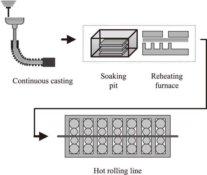
The motivation for this research stems from hot slab scheduling in parallel production lines of the practical Iron-and-Steel Complex. Hot rolling line (HRL) is an operation in which hot slabs are rolled down into hot strip (or plate) steel. As shown in Fig. 1, hot slabs in HRL are supplied by continuous casting (CC) whose task is casting liquid iron into hot slabs one by one. Two middle procedures, heat preservation pit and reheating furnace, are set between CC and HR in order to keep slabs’ temperature fit for hot rolling. The first one is to slow the cooling of hot slabs, the second one is to reheat the slabs so as to make their temperature always satisfy hot rolling temperature restriction. Longer waiting time means more energy needed to reheat the slabs to the ideal rolling temperature. Thus energy loss function is supposed as monotone increasing function dependent of the waiting time.

Fig. 1.

The flow between continuous casting and hot rolling in the Steel-making Complex.

Fig. 2.

The sequence of total primary energy consumption (2002).

Fig. 3.

The difference between practical energy loss curve and the supposed energy loss curve.

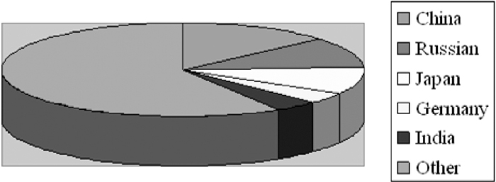
Nowadays, energy crisis has aroused the government and the enterprises’ concern in China. China is the second largest energy producer & consumer in the world, which occupies 22% of the total energy consumption of the whole world in 2002. Iron and Steel industry consumes above 10% of the national total energy consumption, which locates at a priority area in energy conservation. The national output of steel has occupied the first position in the world for 9 years since 1996, but energy consumption of Iron-and-Steel industry is 15%–20% higher than the developed country. Then it is necessary to reduce the energy consumption in order to improve the enterprise’s competitive power.

To reduce the energy loss in hot rolling line, a reasonable schedule of slabs with chain constraints should be determined. The slabs have been formed to several chains in which the order of the slabs has been determined a priori. Then this hot slab scheduling problem can be denoted as P|chains, r_jk, hot|Σf_jk(wait_jk), where wait_jk is the waiting time of slab (j, k) before parallel hot rolling lines, ‘hot’ represents that the slabs arrive with high temperature and f_jk(wait_jk) is the energy loss cost that is dependent on the waiting time of slab (j, k).

The rest of the paper is organized as follows. The review of the related works would be given in section 2. In section 3, we describe and model the hot slabs scheduling problem in parallel hot rolling production lines. The solution procedure for this problem will be presented in sections 4. Section 5 will report the experiment results. Brief conclusions will be given in section 6.

2. Review

Several optimization results about scheduling in iron and steel production have been achieved. Tang et al.¹⁾ focused on a charge batching problem in practice. Tang et al.²⁾ classified the steel-making process problem as a hybrid flowshop problem with complicated technological constraints, and solved the model by Lagrangian relaxation. Tang et al.³⁾ gave four different production processes from continuous casting line to hot rolling line. Generally, most of the slabs still should be reheated before being sent to hot rolling lines, nowadays. Lopez et al.⁴⁾ focused on the production scheduling problem in the hot strip mill, and solved the selection and sequencing problem simultaneously by tabu search. Tang et al.⁵⁾ set up a multiple traveling salesman problem model for hot rolling scheduling without considering time, and got a near-optimal solution by modified genetic algorithm. But they did not consider parallel production lines and chain constraints which differ from our work. Moreover, an exact algorithm is developed in our paper to obtain the optimal solution of the problem.

Previously, parallel machine scheduling problem involved various objective functions and constraints, including minimizing total weighted number of tardy jobs,⁶⁾ minimizing the total weighted completion times,^6,7) maximizing the weight of jobs which meet their respective deadlines,⁸⁾ and minimizing total processing cost⁹⁾ etc. However, the energy consumption is seldom considered, which implies our problem’s innovation.

Batch scheduling for parallel machine scheduling is active topic recently. However, chain constraints were seldom considered in parallel machine scheduling, which determine the order of the items in one chain and the makeup of one chain. Pinedo¹⁰⁾ indicates that P2|chains|ΣC_jk is strongly NP-hard, which is a special case of P|chains, r_jk, hot|Σf_jk(wait_jk). Therefore, P|chains, r_jk, hot|Σf_jk(wait_jk) is also strongly NP-hard, which considers the more complex objective function Σf_jk(wait_jk) and the ready time.

To solve parallel machine scheduling problems, many algorithms have been tried, i.e. dynamic programming,^11,12) heuristic,¹³⁾ column generation,^6,7,14) state space relaxation.^15,16,17,18) However, all the developed algorithms cannot be directly used to solve our problem, since the characteristics of the concerned problem in this paper differs from the previous works at the following several aspects. First of all, the candidate items in our problem are hot slabs with up to about 1200°C, which would incur more costs if they wait in the yard for longer time. Second, the slabs have been formed to several chains in which the slabs have appropriate features so that they can be processed successively without interruption. Third, energy loss cost is set as the objective function of scheduling. At last, parallel hot rolling lines are considered in this paper, and the previous work of scheduling in Iron & Steel Complex usually considers only one production line. To solve our problem optimally, branch and pricing algorithm based on column generation technology is developed in this paper.

3. Problem Description and Modeling

This problem sources from the hot rolling lines. To keep the rolling temperature no lower than a given lower limit, an energy loss cost is incurred by heating the slab. Slabs with similar features are scheduled priori as a chain in which the slabs’ order has been determined. This problem is described as a parallel machine scheduling problem with the objective of minimizing the total energy loss cost while satisfying the chain constraints. Each hot rolling line can roll at most one slab at one time and one slab can also be processed on at most one hot rolling line. It assumed that the time horizon is long enough to complete all the slabs.

Express of energy loss function

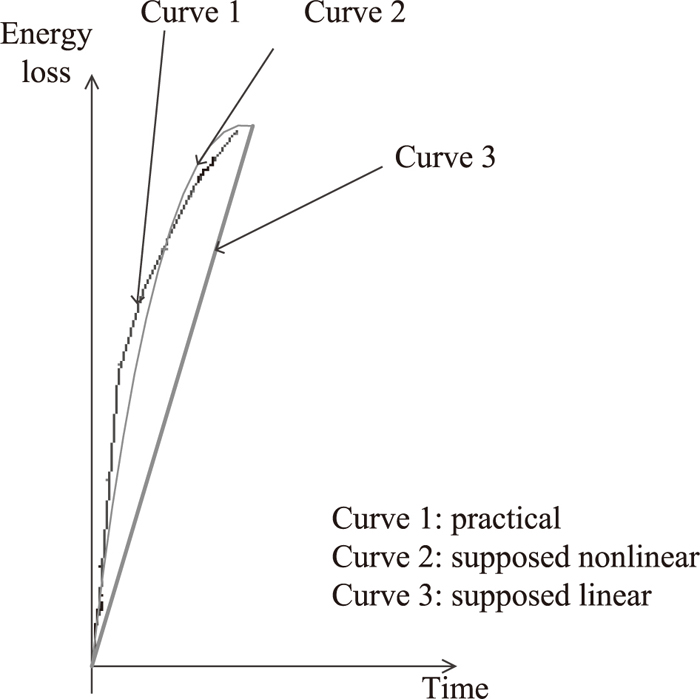
The slab arrives at parallel hot rolling lines with high temperature. The large gap between the room temperature and the slab’s temperature leads to a fast increasing of the slab’s energy loss. The gap decreases as time passed, then the increasing of slab’s energy loss become slower. Based on the analysis, two kinds of energy loss functions are concerned: linear and nonlinear energy loss function, respectively. For the linear case, the energy loss of the k-th slab in chain j - (j, k) is simplified as a linear function of its waiting time with assumed slope ${{\beta }^{\prime }}_{jk}$ (>0). With respect to nonlinear case, the energy loss of slab (j, k) is described as f_jk(wait_jk)= α_jk×wait_jk²+β_jk×wait_jk+γ_jk, where α_jk<0, β_jk>0, γ_jk=0. These two supposed curves can reflect the trend of energy loss’s change in a certain extent.

Notation

M the set of all hot rolling lines, M={1, 2, …, m}, where m is the total number of hot rolling lines.

Ω_c the index set of all chains, Ω_c={1, 2, …, k, …, nc} and the k-th chain is ch_k, chain ch_k contains n_k slabs whose order has been determined a priori by chain constraint. The j-th slab in chain ch_k is slab (j, k). And nc (=|Ω_c|) is the total number of chains.

Ω_s the index set of all concerned chains in schedule s.

N the set of all slabs, there are totally n slabs in this set, then ${\sum }_{k=1}^{nc}{n}_k=n$ .

N_s the set of all concerned slabs in schedule s.

B_jk the set of the slabs that must be processed before slab (j, k) according to the chain precedence constraint corresponding to the chain ch_k.

p_jk the processing time of slab (j, k).

r_jk the ready time of slab (j, k).

Γ_f the set of all feasible acyclic schedules.

Γ_u the set of the schedules in which slabs can be processed more than once.

Decision variables

$x_{ik}=\{\begin{array}{l}\text{1, if the }i\text{-th chain is processed immediately before the }k\text{-th chain.}\\ \text{0, else.}\end{array}$

b_jk the starting time of slab (j, k).

wait_jk the waiting time of slab (j, k).

bc_k the start time of the first slab in ch_k.

Then the hot slab scheduling problem can be formulated as the following master problem and pricing problem. The problem can be solved through the natural interpretation of the master problem and pricing problem.

Master problem:

Define a_ks is the number of times that chain ch_k is processed in schedule s (s∈Γ_f∪Γ_u), f_s is the total energy loss cost of the slabs in the schedule s. Define y_s equals 1 if schedule s (s∈Γ_f∪Γ_u) is used and 0 otherwise. The master problem (MP) is formulated as below.   

$$\mathrm{M}\mathrm{P}\hspace{1em}min\sum _{s\in {\mathrm{\Gamma }}_f\cup {\mathrm{\Gamma }}_u}{f}_s{y}_s$$(1)

subject to   

$$\sum _{s\in {\mathrm{\Gamma }}_f\cup {\mathrm{\Gamma }}_u}{a}_{ks}{y}_s=1,\mathrm{\hspace{0.17em} }\forall k\in {\mathrm{\Omega }}_c$$(2)

  

$$\sum _{s\in {\mathrm{\Gamma }}_f\cup {\mathrm{\Gamma }}_u}{y}_s\le m$$(3)

  

$$y_s\in [0,\mathrm{\hspace{0.17em} }1],\mathrm{\hspace{0.17em} }\forall s\in {\mathrm{\Gamma }}_f\cup {\mathrm{\Gamma }}_u$$(4)

The master problem is completely equivalent to the original concerned problem if all the schedules are involved. Actually, not all the columns are concerned in the solution procedure, so the models in the solution procedure are the restricted version of master problem (RMP). The objective function (1) is minimizing the total energy loss costs of all the slabs. Constraints (2) ensure that each slab is processed exactly once. Constraint (3) represents there are at most m available hot rolling production lines. The RMP is relaxed by relaxing the integer variables y_s to continuous variables in [0, 1]. The dual variables used in the pricing problem can be obtained by solving the relaxed version of RMP.

Pricing problem:

The pricing problem has the task of finding the better column with negative reduced cost. When no columns with negative reduced costs can be found, the optimal solution of the original problem has been obtained. Let π_k, (k∈Ω_c) be the optimal dual solution corresponding to ch_k in constraints (2) and α be the optimal dual solution corresponding to constraint (3). Then the pricing problem can be formulated as follow:   

$$min\mathrm{\hspace{0.17em} }{f}_s-\sum _{k\in {\mathrm{\Omega }}_c}a{}_{ks}\hspace{0.17em}{\pi }_k-\alpha$$(5)

  

$$\sum _{i\in ({\mathrm{\Omega }}_s\backslash \{k\})\cup \left\{0\right\}}{x}_{ik}=\sum _{i\in ({\mathrm{\Omega }}_s\backslash \{k\})\cup \{n+1\}}{x}_{ki},\mathrm{\hspace{0.17em} }\forall k\in {\mathrm{\Omega }}_s$$(6)

  

$$b_{jk}=x_{0k}\sum _{(a,\hspace{0.17em}k)\in B_{jk}}{p}_{ak}+\sum _{i\in {\mathrm{\Omega }}_s\backslash \left\{k\right\}}\left(b{c}_i+\sum _{(a,\hspace{0.17em}k)\in B_{jk}}{p}_{ak}\right)\hspace{0.17em}{x}_{ik},\mathrm{\hspace{0.17em} }\forall (j,\mathrm{\hspace{0.17em} }k)\in N_s$$(7)

  

$$b{c}_k=x_{0k}\sum _{(j,\hspace{0.17em}k)\in c{h}_k}{p}_{jk}+\sum _{i\in {\mathrm{\Omega }}_s\backslash \left\{k\right\}}\left(b{c}_i+\sum _{(j,\hspace{0.17em}k)\in c{h}_k}{p}_{jk}\right)\hspace{0.17em}{x}_{ik},\mathrm{\hspace{0.17em} }\forall k\in {\mathrm{\Omega }}_s$$(8)

  

$$wai{t}_{jk}=b_{jk}-r_{jk},\mathrm{\hspace{0.17em} }\forall (j,\mathrm{\hspace{0.17em} }k)\in N_s$$(9)

  

$$b_{jk}\ge r_{jk},\mathrm{\hspace{0.17em} }\forall (j,\mathrm{\hspace{0.17em} }k)\in N_s$$(10)

  

$$f_s=\sum _{k\in {\mathrm{\Omega }}_c}\left(a_{ks}\times \sum _{(j,\hspace{0.17em}k)\in c{h}_k}{f}_{jk}\left(wai{t}_{jk}\right)\right),\mathrm{\hspace{0.17em} }\forall s\in {\mathrm{\Gamma }}_f\cup {\mathrm{\Gamma }}_u$$(11)

  

$$x_{ik}\in \{0,1\},\mathrm{\hspace{0.17em} }\forall i,\mathrm{\hspace{0.17em} }k\in {\mathrm{\Omega }}_s$$(12)

The objective (5) is to minimize the total reduced costs of schedule s. Constraints (6) mean that the number of the chains processed immediately before chain k equals the numbers of the chains immediately after chain k in the schedule. Constraints (7) and (8) define the starting time of slab (j, k) and the starting time of the k-th chain, respectively. They imply that one production line has no idle time until all the slabs in one chain is finished, once the first slab in one chain is started. Constraints (9) compute the waiting time of slab (j, k). Constraints (10) ensure that each slab (j, k) may not start its processing before its ready time. Constraints (11) determine the total energy loss cost of the slabs in the schedule s. The last constraints (12) define the value range of variables.

The production lines are assumed identical, so the sub-problem is to find a schedule including a subset of slabs in N which satisfies the slab ordering restriction of the problem and the chain constraints, such that the total energy loss cost of the slabs in the schedule s minus the total dual variable value of these slabs is minimized. The pricing problems can be viewed as single machine scheduling problem with chain constraints which should determine the selection and schedule of the slabs simultaneously.

4. Solution Methodology

As it is mentioned before, P|chains, r_jk, hot|Σf_jk(wait_jk) is strongly NP-hard even for the linear case. To obtain the optimal solution of the problem, column generation based algorithm is adopted, which has got better results in solving parallel machine scheduling problem (Chen and Powell⁶⁾ and Vandenakker et al.⁷⁾). In column generation procedure, the master problem and the pricing problem are solved iteratively. The linear relaxation of RMP is solved to provide dual variables to pricing problem, and the pricing problem is solved to find out the schedule which can further reduce the objective of the RMP. While the pricing problem cannot find the schedule with negative reduced costs, the linear version of the master problem is optimally solved, and a lower bound is obtained. Then the original problem is optimally solved by so-called branch and pricing algorithm, which combines the column generation technology and branch & bound. Consequently, the key elements in our algorithm are given.

4.1. Solution Strategy of Pricing Problem

The pricing problem is strongly NP-hard because its objective is more complex than 1|r_jk,|ΣC_jk which is mentioned strongly NP-hard in Pindedo.¹⁰⁾ To solve it, a dynamic programming formulation based on state space relaxation with 2-cycles elimination is proposed.

The optimal solution of the pricing problem corresponds to state (S, t) representing the schedule that the slabs in the chains of S are scheduled exactly once in it and the processing terminates at time t, when S is the set including all the concerned chains. Let F(S, t) be the minimum cost of state (S, t). Then the pricing problem can be solved by the following recursion (13).   

$$\begin{array}{l}F(S,t)=\\ \{\begin{array}{l}\underset{i\in S}{min}\left\{F\left(S-\left\{i\right\},t-\sum _{(j,\hspace{0.17em}i)\in c{h}_i}{p}_{ji}\right)+\sum _{(j,\hspace{0.17em}i)\in c{h}_i}{f}_{ji}\left(t-\sum _{(a,\hspace{0.17em}i)\in c{h}_i\backslash B_{ji}}{p}_{ai}-r_{ji}\right)-{\pi }_i\right\},\\ \mathrm{\hspace{0.17em} }\mathrm{i}\mathrm{f}\mathrm{\hspace{0.17em} }t\in \left[R_i+P_i-1,\hspace{0.17em}{D}_i\right]+\infty ,\hspace{1em}\hspace{1em}\hspace{1em}\hspace{1em}\hspace{1em}\hspace{1em}\hspace{1em}\hspace{1em}\hspace{1em}\hspace{1em}\hspace{1em}\hspace{1em}\hspace{1em}\hspace{1em}\hspace{1em}\hspace{1em}\hspace{1em}\hspace{1em}\hspace{1em}\hspace{1em}\hspace{1em}\hspace{1em}\text{otherwise}\end{array}\end{array}$$(13)

The number of the states for the above recursion is O(T2^cn) where T is the length of planning period. Thus the computation time of the recursion is exponential. To reduce the computation time, the state (S, t) has to be relaxed to (k, t) which represents the schedule that the k-th chain is scheduled last and finished at time t. In the relaxed state space, there are cnT states concerned, therefore, the solution of the pricing problem is accelerated. At the expense, some non-feasible paths of the pricing problem, in which one slab can be processed more than once can also be generated by solving the pricing problem. Thus the lower bound of the pricing problem is found instead of the optimal solution.

To tighten the lower bound, 2-cycles elimination is proposed, which can avoid one chain is processed twice consecutively. Let F(k, t) be the minimum cost of the schedule that the k-th chain is scheduled last in the current sequence and finished at time t. Let F¹(i, t) be the objective function value of the schedule with minimum cost that the last processed chain is ch_i and the processing is terminated no later than time point t. Let F²(i, t) be the objective function value of the schedule with second minimum cost that the last processed chain is ch_i, the processing is terminated no later than time point t and ω¹(i, t) ≠ ω²(i, t) where ω^η(i, t) is the chain that is processed immediately before chain i in the schedule corresponding to F^η(i, t). Then the pricing problem can be solved by the following recursion (14).   

$$\begin{array}{l}F(k,\mathrm{\hspace{0.17em} }t)=\underset{i\in ({\mathrm{\Omega }}_c\backslash \{k\})\cup \left\{0\right\}}{min}\\ \left\{F^{\eta }\left(i,\mathrm{\hspace{0.17em} }t-\sum _{(a,\hspace{0.17em}k)\in c{h}_k}{p}_{ak}\right)+\sum _{(j,\hspace{0.17em}k)\in c{h}_k}{f}_{jk}\left(t-\sum _{(a,\hspace{0.17em}k)\in c{h}_k\backslash B_{jk}}{p}_{ak}-r_{jk}\right)-{\pi }_k\right\},\mathrm{\hspace{0.17em} }\\ \mathrm{i}\mathrm{f}\mathrm{\hspace{0.17em} }t\in \left[R_k+P_k-1,\hspace{0.17em}{D}_k\right],\mathrm{\hspace{0.17em} }k\in {\mathrm{\Omega }}_c\end{array}$$(14)

where η is equal to 1 if ${\omega }^1\left(i,\mathrm{\hspace{0.17em} }t-\sum _{(a,\hspace{0.17em}k)\in c{h}_k}{p}_{ak}\right)\ne k$ , 2 otherwise. F¹(k, t) and F²(k, t) are computed by the following recursions.   

$$F^1(k,\mathrm{\hspace{0.17em} }t)=\underset{t\le t}{min}\left\{F(k,\mathrm{\hspace{0.17em} }t)\right\},\mathrm{\hspace{0.17em} }\mathrm{f}\mathrm{o}\mathrm{r}\mathrm{\hspace{0.17em} }k\in {\mathrm{\Omega }}_c,\mathrm{\hspace{0.17em} }C{R}_k+C{P}_k-1\le t\le D_k$$(15)

  

$$\begin{array}{l}{F}^2(k,\mathrm{\hspace{0.17em} }t)=\underset{t\le t}{min}\left\{F(k,\mathrm{\hspace{0.17em} }t)|\omega (k,\mathrm{\hspace{0.17em} }t)\ne {\omega }^1(k,\mathrm{\hspace{0.17em} }t)\right\},\mathrm{\hspace{0.17em} }\\ \mathrm{f}\mathrm{o}\mathrm{r}\mathrm{\hspace{0.17em} }k\in {\mathrm{\Omega }}_c,\mathrm{\hspace{0.17em} }C{R}_k+C{P}_k-1\le t\le D_k\end{array}$$(16)

where R_k is the earliest start time of the k-th chain which is computed by $R_k=\underset{(j,\hspace{0.17em}k)\in c{h}_k}{max}\left\{r_{jk}-\sum _{(a,\hspace{0.17em}k)\in B_{jk}}{p}_{ak}\right\}$ , such that the slabs in ch_k can be processed without time gap if the first slab in this chain is not started before R_k; P_k is the time to process all the slabs in the k-th chain serially and $P_k=\sum {\hspace{0.17em}}_{(j,\hspace{0.17em}k)\in c{h}_k}{p}_{jk}$ ; any chain ch_k (k∈Ω_c) can be completed no later than D_k in an optimal schedule. The computation of D_k would be given later. The recursion (14) remains the same complexity of O(cn²max{D_k}) at the worst case.

In order to determine the plan period of the recursion procedure, D_k is calculated for each chain k (k∈Ω_c), such that chain k cannot be finished after D_k in the optimal solution. Then the whole plan must be finished before max_k∈_Ωc {D_k }. For any chain k∈Ω_c, D_k is computed by   

$$D_k=max\left\{R_k,\mathrm{\hspace{0.17em} }{max}_{i\in {\mathrm{\Omega }}_c\backslash \left\{k\right\}}\left\{R_i\right\}+\lfloor \frac{\sum _{i\in {\mathrm{\Omega }}_c\backslash \left\{k\right\}}{P}_i}{m}\rfloor -\sum _{i=1}^{\nu }{\rho }_i{P}^{min}\right\}+P_k,$$(17)

where ρ_i is a variable indicating whether the plan period can be shortened by arranging m chains processed during [(i-1)P^max, iP^max). P^min and P^max are the minimum and maximum processing time among the chains that can be finished before $ma{x}_{i\in {\mathrm{\Omega }}_c\backslash \left\{k\right\}}\left\{R_i\right\}$ , respectively. And the time horizon can be shortened at most νP^min. The computation of these four parameters is given as follow.   

$${\rho }_i=\{\begin{array}{l}1,\mathrm{\hspace{0.17em} }\mathrm{i}\mathrm{f}\mathrm{\hspace{0.17em} }{\delta }_{i-1}-\sum _{k=1}^{i-1}{\rho }_{k}m\ge m\\ 0,\mathrm{\hspace{0.17em} }\mathrm{e}\mathrm{l}\mathrm{s}\mathrm{e}\end{array}\mathrm{\hspace{0.17em} },$$

  

$$P^{min}=\underset{R_g<{max}_{i\in {\mathrm{\Omega }}_c\backslash \left\{k\right\}}\left\{R_i\right\}-P_g}{min}\left\{P_g\right\},$$

  

$$P^{max}=\underset{R_g<{max}_{i\in {\mathrm{\Omega }}_c\backslash \left\{k\right\}}\left\{R_i\right\}-P_g}{max}\left\{P_g\right\},$$

  

$$\nu =\lfloor \frac{\underset{i\in {\mathrm{\Omega }}_c\backslash \left\{k\right\}}{max}\left\{R_i\right\}}{P^{max}}\rfloor .$$

To make the computation of D_k clearly, the definition of δ_i is given as the number of chains whose earliest start time R_g∈[0, iP^max), for $g\in {\mathrm{\Omega }}_c\backslash \left\{k\right\}$ . Especially, δ₀ involves the chains arriving at zero. Expression (17) is explained as follow with the assumption that the cost corresponding to chain ch_k becomes larger as it completes later.

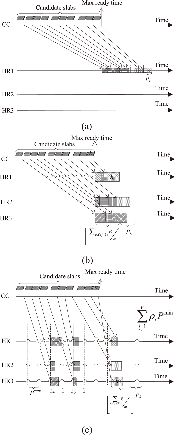
In the worst case, all the chains of slabs are processed before the k-th chain on one hot rolling line (as Fig. 4(a)), which means   

$$C_k\le \underset{i\in {\mathrm{\Omega }}_c}{max}\left\{R_i\right\}+\sum _{i\in {\mathrm{\Omega }}_c}{P}_i.$$(18)

Fig. 4.

The range of a slab’s largest completion time.

In addition, an extreme case is considered in which the k-th chain is scheduled last in the optimal schedule. If the k-th chain is removed from the optimal schedule, a new schedule is obtained. Let the first completed production line in the new schedule is released at time point C_min (as Fig. 4(b)). Then it is obviously   

$$C_{min}\le \underset{i\in {\mathrm{\Omega }}_c\backslash \left\{k\right\}}{max}\left\{R_i\right\}+\lfloor \frac{\sum _{i\in {\mathrm{\Omega }}_c\backslash \left\{k\right\}}{P}_i}{m}\rfloor ,$$(19)

in which all the slabs are processed after $ma{x}_{i\in {\mathrm{\Omega }}_c\backslash \left\{k\right\}}\left\{R_i\right\}$ .

Furthermore, there must be some slabs finished before $ma{x}_{i\in {\mathrm{\Omega }}_c\backslash \left\{k\right\}}\left\{R_i\right\}$ in the optimal schedule, otherwise a better schedule can be obtained by arranging ${\sum }_{i=1}^{\nu }m{\rho }_i$ slabs belonging to set $\left\{g|g\in {\mathrm{\Omega }}_c\backslash \left\{\mathrm{k}\right\},\mathrm{\hspace{0.17em} }{R}_g+P_g\le \underset{i\in {\mathrm{\Omega }}_c\backslash \left\{k\right\}}{max}\left\{R_i\right\}\right\}$ to be finished before time point $ma{x}_{i\in {\mathrm{\Omega }}_c\backslash \left\{k\right\}}\left\{R_i\right\}$ (as Fig. 4(c)).

The inequality can be tightened as   

$$C_{min}\le \underset{i\in {\mathrm{\Omega }}_c\backslash \left\{k\right\}}{max}\left\{R_i\right\}+\lfloor \frac{\sum _{i\in {\mathrm{\Omega }}_c\backslash \left\{k\right\}}{P}_i}{m}\rfloor -\sum _{i=1}^{\nu }{\rho }_i{P}^{min}.$$(20)

in which ${\sum }_{i=1}^{\nu }{\rho }_i{P}^{min}$ is subtracted from the right item of (19) because at least ${\sum }_{i=1}^{\nu }m{\rho }_i$ slabs can be finished before $\underset{i\in {\mathrm{\Omega }}_c\backslash \left\{k\right\}}{max}\left\{R_i\right\}$ instead of after it and these slabs’ processing time is no less than P^min. Then the releasing of each machine can be preacted at least $\frac{\sum _{i=1}^{\nu }m{\rho }_i}{m}\times P^{min}$ . Then the completion time of chain k should satisfy the following inequality,   

$$C_k\le max\left\{R_k,\mathrm{\hspace{0.17em} }\underset{i\in {\mathrm{\Omega }}_c\backslash \left\{k\right\}}{max}\left\{R_i\right\}+\lfloor \frac{\sum _{i\in {\mathrm{\Omega }}_c\backslash \left\{k\right\}}{P}_i}{m}\rfloor -\sum _{i=1}^{\nu }{\rho }_i{P}^{min}\right\}+P_k$$(21)

Otherwise, a better result can be obtained by arranging the slabs in chain k processed at the last position of the first completed production line corresponding to C_min.

4.2. Branching Strategy

If the optimal solution of the linear relaxation problem at root node does not satisfy the integer condition, branching is needed to find the optimal solution of the original problem. Here adopt the following branching strategy based on the most fractional relationship between two chains. For a node in the branching tree that has been explored, if the solution of linear relaxation problem is fractional, an appropriate fractional relationship between two chains i and k is then selected to branch on next. Two child nodes are created. For the left child node, it restricts that chain i cannot be processed immediately before chain k. For the right child node, it requires that chain i must be processed immediately before chain k

With respect to the case of linear energy loss function, a lemma is proposed to reduce the branching feasibilities. Because the energy loss function of slab (j, k) is a linear function, which can be expressed as f_jk(wait_jk)= ${{\beta }^{\prime }}_{jk}$ ×wait_jk+ γ_jk, so it has additivity property.

Lemma 1: In the optimal solution, chain i can not be scheduled immediately before chain k, if ${\sum }_{(j,\hspace{0.17em}i)\in c{h}_i}{f}_{ji}\left(P_k\right)-{\sum }_{(j,\hspace{0.17em}k)\in c{h}_k}{f}_{jk}\left(P_i\right)<0$ .

Proof: The lemma is proven by contradiction. Suppose that chains i is processed immediately before chain k in the optimal solution. The objective function value can be written as   

$$\begin{array}{l}O=\sum _{g\in {\mathrm{\Omega }}_c\backslash \{i,\hspace{0.17em}k\}}\sum _{(j,\hspace{0.17em}g)\in c{h}_g}{f}_{jg}\left(wai{t}_{jg}\right)\\ +\sum _{(j,\hspace{0.17em}i)\in c{h}_i}{f}_{ji}\left(wai{t}_{ji}\right)+\sum _{(j,\hspace{0.17em}k)\in c{h}_k}{f}_{jk}\left(wai{t}_{jk}\right)\end{array}$$

The objective function value of the case that exchange chains i and k is written as   

$$\begin{array}{l}{O}^{\prime }=\sum _{g\in {\mathrm{\Omega }}_c\backslash \{i,\hspace{0.17em}k\}}\sum _{(j,\hspace{0.17em}g)\in c{h}_g}{f}_{jg}\left(wai{t^{\prime }}_{jg}\right)\\ +\sum _{(j,\hspace{0.17em}i)\in c{h}_i}{f}_{ji}\left(wai{t^{\prime }}_{ji}\right)+\sum _{(j,\hspace{0.17em}k)\in c{h}_k}{f}_{jk}\left(wai{t^{\prime }}_{jk}\right),\end{array}$$

where wait′_jg = wait_jg for (j, g)∈ch_g, $g\in {\mathrm{\Omega }}_c\backslash \{i,\hspace{0.17em}k\}$ ; $wai{t^{\prime }}_{ji}-wai{t}_{ji}={\sum }_{(a,\hspace{0.17em}k)\in c{h}_k}{p}_{ak}$ for (j, i)∈ch_i; $wai{t^{\prime }}_{jk}-wai{t}_{jk}=-{\sum }_{(a,\hspace{0.17em}i)\in c{h}_i}{p}_{ai}$ for (j, k)∈ch_k .

Then $O^{\prime }-O=\sum _{(j,\hspace{0.17em}i)\in c{h}_i}{f}_{ji}\left(\sum _{(a,\hspace{0.17em}k)\in c{h}_k}{p}_{ak}\right)\mathrm{\hspace{0.17em} }\hspace{0.17em}-\sum _{(j,\hspace{0.17em}k)\in c{h}_k}{f}_{jk}\left(\sum _{(a,\hspace{0.17em}i)\in c{h}_i}{p}_{ai}\right)$ because of the additivity property.

Since the former case is the optimal solution, $\sum _{(j,\hspace{0.17em}i)\in c{h}_i}{f}_{ji}\left(\sum _{(a,\hspace{0.17em}k)\in c{h}_k}{p}_{ak}\right)-\sum _{(j,\hspace{0.17em}k)\in c{h}_k}{f}_{jk}\left(\sum _{(a,\hspace{0.17em}i)\in c{h}_i}{p}_{ai}\right)\ge 0$ . It leads a contradiction, then the proof is completed.

For the problem whose energy loss function is linear, some feasible branching satisfying the condition of lemma 1 can be excluded because the optimal solution cannot exist in the child nodes generated after this kind branching.

4.3. Heuristic to Get The Initial Solution

Some initial columns must be generated to start the column generation procedure. The heuristic in Park and Kim¹⁴⁾ is used to obtain the initial solution of parallel machine scheduling.

5. Computation Experiments

The above two algorithm are implemented by C language and tested on a Pentium IV with 3.0 GHz PC. The computation experience is reported to illustrate the performance of the the column generation algorithms. Linear programming problem inside the column generation algorithms are solved by IBM OSL, a commercial LP solver.

5.1. Experiment Design

The size parameters are given as follow.

Number of slabs: n∈{60, 80, 100, 120}.

Number of production lines: m∈{3, 5, 6, 8}.

Number of chains: cn∈{20, 30, 40, 50, 60}.

Processing time (p_jk) is an integer number uniformly drawn from [1, 10]. A schedule is constructed by selecting slabs (j, k) at random and then scheduling them at the earliest possible time t_i. Ready times is set as r_jk =t_i – U[1, 30], where random numbers are integer-valued. Adjustments are made to avoid negative ready times for the first slabs by increasing all schedule times t_i.

Parameters to determine energy loss function.

-linear case ( ${{\beta }^{\prime }}_{jk}$ ). It is an integer number uniformly drawn from [1, 1000].

-nonlinear case (α_jk, β_jk, γ_jk). Firstly, α_jk is an integer number uniformly drawn from [-10, -1]. β_jk is set as -2α_jk(D_k-r_jk) in order to keep that the later the slab is processed, the larger the energy loss is. The determination of parameter β_jk is based on the following analysis. The temperature of the slab (j, k) cannot be less than room temperature based on heat exchange theory. Meanwhile the minimum reachable temperature of the slab (j, k) at the parabola’s extreme point is assumed to correspond to the difference between D_k and the ready time r_jk. γ_jk must be zero because there is no energy loss when slab (j, k) arrives just now.

5.2. Computational Results

The following two tables report the computational results for the problems with linear energy loss function and the problem with nonlinear energy loss function, respectively. The problem is determined by the parameters in the first three columns n, m, cn where n is the number of slabs, m is the number of parallel hot rolling lines and cn is the number of chains. The fourth column represents the average integrality gap, the integrality gap is equal to the ratio of the difference between the optimal solution and the lower bound to the lower bound, which is used to evaluate the performance of the lower bound. The fifth column represents the average computation time for solving these problems. The sixth column gives the number of the instances that is solved at root node. The last column represents the average number of the nodes in the solution procedure.

From Tables 1 and 2, the hot slab scheduling problems for both of the cases that the energy loss function is linear and nonlinear can be solved with up to 120 slabs and 60 chains in a reasonable time.

Table 1. Computational results in the case of linear energy loss function.

Problem			Integrality Gap (%)	Time (s)	rnobran	B&B nodes
n	cn	m
60	20	3	0.0025%	3.8405	15/20	1.35
60	20	5	0.0095%	1.6200	16/20	1.25
60	30	3	0.0000%	17.1055	20/20	1.00
60	30	5	0.0095%	7.8030	13/20	1.70
60	30	6	0.0395%	5.1655	13/20	2.05
80	20	3	0.0000%	5.8535	19/20	1.10
80	20	5	0.0005%	2.3160	17/20	1.20
80	40	3	0.0025%	98.4845	15/20	3.95
80	40	5	0.0020%	30.4745	16/20	2.00
80	40	8	0.0045%	14.014	11/20	2.65
100	20	3	0.0000%	6.7010	20/20	1.00
100	20	5	0.0020%	2.7520	16/20	1.65
100	50	5	0.0050%	103.9345	8/20	3.85
100	50	6	0.0030%	68.8880	16/20	5.45
100	50	8	0.0030%	47.1780	12/20	3.8
120	30	3	0.0010%	41.5885	16/20	1.80
120	30	5	0.0000%	17.2625	16/20	1.80
120	30	6	0.0000%	11.9380	14/20	1.80
120	40	3	0.0000%	125.0730	18/20	1.60
120	40	5	0.0115%	51.2035	13/20	1.75
120	40	8	0.0000%	24.6050	17/20	1.20
120	60	5	0.0004%	228.8056	5/20	4.70
120	60	6	0.0000%	121.3305	7/20	7.53
120	60	8	0.0045%	92.5355	11/20	5.05
120	60	10	0.0010%	64.4000	11/20	5.80

Table 2. Computational results in the case of nonlinear energy loss function.

Problem			Integrality Gap (%)	Time (s)	rnobran	B&B nodes
n	cn	m
60	20	3	0.0095%	1.3555	11/20	2.75
60	20	5	0.0315%	0.5105	13/20	1.85
60	30	3	0.0030%	6.2110	13/20	2.20
60	30	5	0.0085%	3.0220	7/20	3.85
60	30	6	0.0070%	2.4385	3/20	5.45
80	20	3	0.0000%	1.4555	18/20	1.10
80	20	5	0.0045%	0.6520	12/20	1.95
80	40	3	0.0000%	32.4415	7/20	5.55
80	40	5	0.0070%	11.8965	6/20	6.40
80	40	8	0.0005%	4.7000	5/20	4.65
100	20	3	0.0000%	1.9765	14/20	1.50
100	20	5	0.0155%	0.8365	11/20	2.05
100	50	5	0.0040%	48.7250	7/20	5.60
100	50	6	0.0005%	37.7590	5/20	7.15
100	50	8	0.0005%	25.0915	6/20	8.55
120	30	3	0.0000%	11.6515	17/20	3.10
120	30	5	0.0000%	5.3430	11/20	3.55
120	30	6	0.0000%	3.5255	13/20	2.30
120	40	3	0.0010%	32.8280	12/20	2.00
120	40	5	0.0015%	16.3095	3/20	6.05
120	40	8	0.0050%	7.8855	6/20	8.15
120	60	5	0.0010%	100.6900	0/20	12.25
120	60	6	0.0020%	65.6125	1/20	10.15
120	60	8	0.0000%	34.8530	2/20	8.85
120	60	10	0.0000%	27.5550	2/20	11.75

When the number of the chains is smaller, or the number of production lines is larger, the computation time is shorter. The computational time is insensitive with the number of the slabs. This probably can be explained by that the problem pays more attention to the scheduling of the chains, and the order of the slabs in one chain has been determined by the chain constraints, so the factors inflecting the algorithm complexity is in fact the number of the chains. This is to say that the algorithm is good at the slab scheduling problem with less varieties.

For the case whose energy loss function is linear, most instances can be solved at the root node from Table 1. The ratio of the instances that is solved at root node becomes less for the case whose energy loss function is nonlinear. The small integrality gap in the experimental results illustrate that our proposed algorithm can achieve a tight lower bound, which can be obtained at the root node.

From Tables 1 and 2, the objective functions have week influences to the results of the algorithms except the average node number. This may be because a lemma is proposed in the linear case such that some nodes that cannot generate optimal solution are eliminated. For the other aspects, the energy loss function does not relate to the algorithm framework no matter for the linear case or for the nonlinear case. The energy loss function is just used to evaluate the schedule.

6. Conclusion

This paper studies the problem that determines the schedule of the hot slabs in parallel hot rolling production lines in which chain constraints are concerned, the objective function is minimizing the total energy loss costs. In this paper, two cases of the objective functions are concerned including the linear and nonlinear energy loss function. The problem can be classified to P|chains, r_jk, hot|Σf_jk(wait_jk). Since it is strongly NP-hard, column generation combined with branch and bound is used to obtain the exact solutions of this problem. The experimental results illustrate that the proposed algorithm can optimally solve the medium scale instances with both linear and nonlinear energy loss function.

Acknowledgement

This research is partly supported by National Natural Science Foundation (Grant No. 71402020, 61374207), National 863 High-Tech Research and Development Program of China (2013AA040704).

References

• 1)   L. X.  Tang,  G. S.  Wang and  Z. L.  Chen: Oper. Res., 62 (2014), 772.
• 2)   L. X.  Tang,  P. B.  Luh,  J. Y.  Liu and  L.  Fang: Int. J. Prod. Res., 40 (2002), 55.
• 3)   L. X.  Tang,  J. Y.  Liu,  A. Y.  Rong and  Z. H.  Yang: Eur. J. Oper. Res., 133 (2001), 1.
• 4)   L.  Lopez,  M. W.  Carter and  M.  Gendreau: Eur. J. Oper. Res., 106 (1998), 317.
• 5)   L. X.  Tang,  J. Y.  Liu,  A. Y.  Rong and  Z. H.  Yang: Eur. J. Oper. Res., 124 (2000), 267.
• 6)   Z. L.  Chen and  W. B.  Powell: Networks, 11 (1999), 78.
• 7)   J. M.  Vandenakker,  J. A.  Hoogeveen and  S. L.  Vandevelde: Oper. Res., 47 (1999), 862.
• 8)   A.  Bar-Noy,  S.  Guha,  J.  Naor and  B.  Schieber: SIAM J. Comput., 31 (2001), 331.
• 9)   V.  Jain and  I. E.  Grossmann: INFORMS J. Comput., 13 (2001), 258.
• 10)   M.  Pindedo: Scheduling: Theory, Algorithms, and Systems, 2nd ed., Tsinghua University Press, Beijing, (2005), 35.
• 11)   T. C. E.  Cheng,  Z. L.  Chen,  M. Y.  Kovalyov and  B. M. T.  Lin: IIE Trans., 28 (1996), 953.
• 12)   S.  Webster and  M.  Azizoglu: Comput. Oper. Res., 28 (2001), 127.
• 13)   M. W.  Park and  Y. D.  Kim: Comput. Ind. Eng., 33 (1997), 793.
• 14)   Z. L.  Chen and  W.  Powell: Naval Res. Logist., 50 (2003), 823.
• 15)   E.  Choi and  D.  Tcha: Comput. Oper. Res., 34 (2007), 2080.
• 16)   N.  Christofides,  A.  Mingozzi and  P.  Toth: Networks, 11 (1981), 145.
• 17)   T. S.  Abdul-Razaq and  C. N.  Potts: J. Oper. Res. Soc., 39 (1988), 141.
• 18)   T.  Ibaraki and  Y.  Nakamura: Eur. J. Oper. Res., 76 (1994), 72.