Transient Fluid Flow during Steady Continuous Casting of Steel Slabs: Part II. Effect of Double-Ruler Electro-Magnetic Braking

Abstract

Plant measurements and computational models of transient flow with and without electromagnetic fields are applied to investigate transient phenomena in the nozzle and mold region during nominally steady steel slab casting. In Part II of this two-part article, the effect of applying a static magnetic field on stabilizing the transient flow is investigated by modeling a double-ruler Electro-Magnetic Braking (EMBr) system, under conditions where measurements were obtained. A Reynolds Averaged Navier-Stokes (RANS) computational model using the standard k–ε model is employed with a magnetic field distribution extrapolated from measurements. The magnetic field decreases velocity fluctuations and deflects the jet flow downward in the mold, resulting in a flatter surface level and slower surface flow with slightly better stability. The effect of EMBr on surface level and surface velocity, including the effect of the real conducting steel shell, falls between the cases assuming perfectly-conducting and insulating walls. Measurements using an eddy current sensor and nail boards were performed to quantify the effect of EMBr on level and velocity at the mold surface. Power spectrum analysis of the surface level variations measured by the sensor revealed a frequency peak at ~0.03 Hz (~35 seconds) both with and without the EMBr. With EMBr, the surface level is more stable, with lower amplitude fluctuations, and higher frequency sloshing. The EMBr also produced ~20% lower surface velocity, with ~60% less velocity variations. Finally, the motion of the slag-steel interface level causes mainly lifting rather than displacement of the molten slag layer, especially near the SEN.

1. Introduction

To control surface level and velocity to avoid defects in steel slab continuous casting, many efforts have been made to optimize nozzle geometry and caster operating conditions including casting speed, submergence depth of the nozzle, mold width, argon gas injection, and Electro-Magnetic Forces (EMF), with the aim to achieve stable mold flow under nominally steady-state operation conditions. Application of a magnetic field to stabilize steel flow is an attractive method because the induced forces intrinsically adjust to flow variations. The field strength distribution depends on the magnet position(s), coil windings, and current. Electromagnetic systems are classified according to the type of field: static (DC current) or moving field (usually AC current). Static systems include local, single-ruler, and double-ruler (FC-Mold) Electro-Magnetic Braking (EMBr). Moving systems include Electro-Magnetic Level Stabilizer (EMLS), Electro-Magnetic Level Accelerator (EMLA), and Electro-Magnetic Rotating Stirrer (EMRS). EMBr is often used in slab continuous casting.

Many previous studies have investigated the average effect of EMBr on steady-state fluid flow in the mold.^{1,2,3,4,5,6,7,8,9,10,11)} For example, Cukierski and Thomas reported that local EMBr usually decreases the surface velocity, depending on the submergence depth of the Submerged Entry Nozzle (SEN).⁸⁾ Wang and Zhang investigated the effects of local EMBr on the fluid flow, heat transfer, and transport of argon bubbles and inclusions in the mold.⁹⁾ Li et al. studied the effect of double-ruler EMBr with argon gas injection on mold flow¹⁰⁾ and biased flow induced by nozzle misalignment.¹¹⁾ Only a few previous studies have investigated the effect of EMBr on transient flow and flow stability.^{12,13,14,15,16,17)} Timmel et al. found that single-ruler EMBr across the nozzle port induces significant jet fluctuations with non-conducting mold walls, and efficient damping of jet fluctuations in the conducting mold through measuring mold flow in a GaInSn physical model using Ultrasound Doppler Velocimetry (UDV).^12,13) Chaudhary et al. and Singh et al. performed Large Eddy Simulation (LES) of the GaInSn physical model and found that positioning a strong single-ruler EMBr across the nozzle port region induces large-scale and low frequency flow variations.^14,15) Singh et al. also observed that the single-ruler EMBr across the nozzle induces higher surface velocity, surface level, and surface level fluctuations by deflecting the jet flow upward, and the large scale jet wobbling induced by the EMBr with insulating wall is decreased with the EMBr with conducting wall.¹⁵⁾ These LES models predict that double-ruler EMBr causes surface velocity and velocity variations both decrease greatly.^14,17)

Part I of this two-part article presented models and experimental methods, and applied them to investigate two-phase transient flow.¹⁸⁾ In Part II, the effect of double-ruler EMBr on transient flow in a conventional steel slab continuous caster is investigated using both computational modeling and plant measurements. Turbulent flow in the nozzle and mold are computed by solving the standard Magneto-Hydro-Dynamics (MHD) flow equations. Plant measurements were conducted using an eddy current sensor as shown in Fig. 1 and nail boards to quantify the effect of EMBr on surface level, surface flow, and the slag pool thickness. Furthermore, the effect of EMBr on stability of surface level and velocity is investigated. Details of the nozzle geometry and casting conditions were given in Table 1 of Part I.¹⁸⁾

Fig. 1.

Position of eddy current sensor in the mold. (Online version in color.)

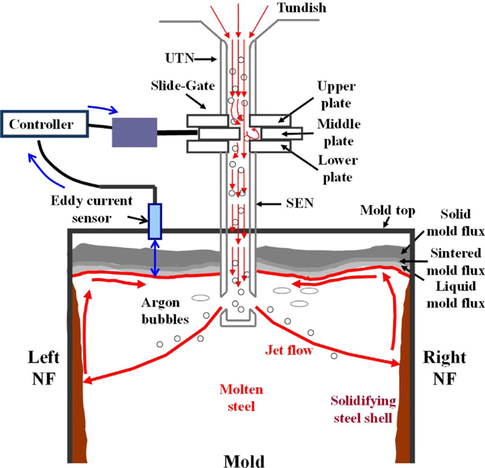
Table 1. Process parameters.

Casting speed	1.7 m/sec
Domain width	650 mm
Domain thickness	250 mm
Domain length	4648 mm (mold region: 3000 mm)
Molten steel density	7000 kg/m3
Molten steel visocity	0.0067 kg/ms
Electrical conductivity of molten steel	714000 (Ωm)–1
Electrical conductivity of solid shell	787000 (Ωm)–1

2. External Magnetic Field Distribution

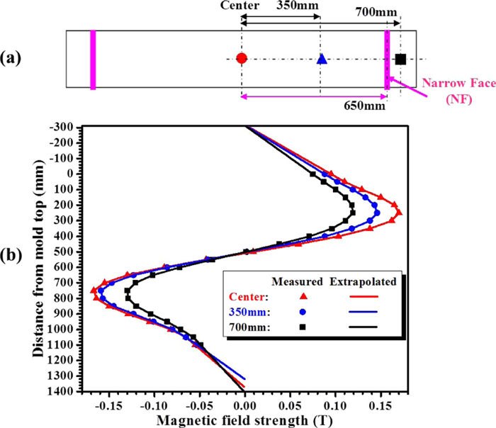
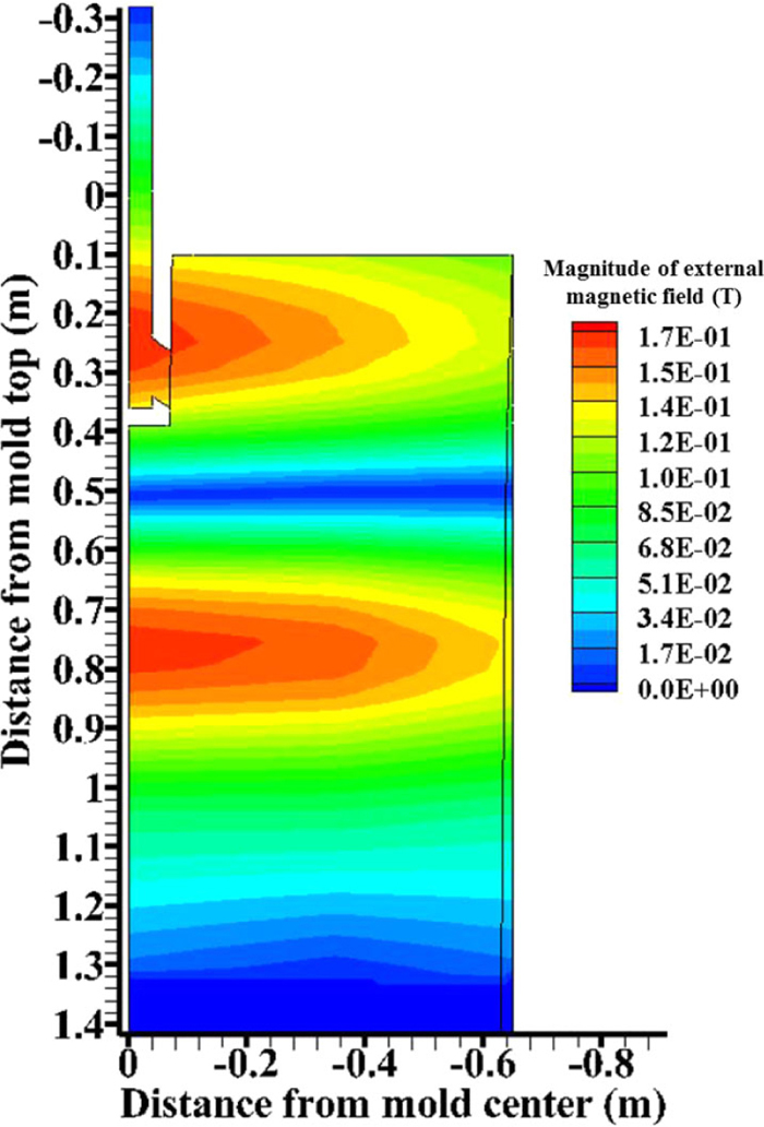
The magnetic field was measured at 69 data points in the mold cavity as explained in Part I.¹⁸⁾ The magnetic field applied by the double-ruler EMBr is shown in Fig. 2, and has high peaks in two regions: one centered just above the port, ~250 mm below mold top and the other below the nozzle port, ~750 mm below mold top. The magnetic field strength decreases significantly towards to the Narrow Face (NF). The measurements were extrapolated to produce the full 3D magnetic field distribution including the nozzle region and deep into the strand. The external magnetic field implemented to the computational model is visualized in Fig. 3.

Fig. 2.

External EMBr field: (a) locations measured, and (b) magnetic field profiles. (Online version in color.)

Fig. 3.

External magnetic field magnitude distribution in the nozzle and mold. (Online version in color.)

3. Computational Model

A three-dimensional finite-volume computational model employing a Reynolds Averaged Navier-Stokes (RANS) approach using the standard k–ε model coupled with a MHD model is applied to predict molten steel flow field in the nozzle and mold regions with the double-ruler EMBr. Steady-state single-phase flow was first predicted by the standard k–ε model and then, the coupled MHD model system was applied to calculate the effect of the EMBr. The equations and boundary conditions were solved with the finite-volume method in ANSYS FLUENT, as described in Part I.¹⁸⁾

3.1. MHD Model

A Lorentz force source term ${\overrightarrow{\mathrm{F}}}_{\mathrm{L}}$ is added to the RANS model Eqn. 7 of Part I,¹⁸⁾ as given by   

$${\overrightarrow{\mathrm{F}}}_{\mathrm{L}}=\overrightarrow{\mathrm{j}}\times \left({\overrightarrow{\mathrm{B}}}_0+\overrightarrow{\mathrm{b}}\right)$$(1)

where ${\overrightarrow{\mathrm{B}}}_0$ is the applied external magnetic field, $\overrightarrow{\mathrm{b}}$ is the induced magnetic field, and $\overrightarrow{\mathrm{j}}$ is induced current density, calculated by   

$$\overrightarrow{\mathrm{j}}=\frac{1}{\mu }\nabla \times \left({\overrightarrow{\mathrm{B}}}_0+\overrightarrow{\mathrm{b}}\right)$$(2)

where μ is magnetic permeability of the molten steel and $\overrightarrow{\mathrm{b}}$ is calculated from the magnetic induction equation:   

$$\frac{\partial \overrightarrow{\mathrm{b}}}{\partial \mathrm{t}}+\left(\overrightarrow{\mathrm{u}}\cdot \nabla \right)\overrightarrow{\mathrm{b}}=\frac{1}{\mu \sigma }{\nabla }^2\overrightarrow{\mathrm{b}}+\left[\left({\overrightarrow{\mathrm{B}}}_0+\overrightarrow{\mathrm{b}}\right)\cdot \nabla \right]\overrightarrow{\mathrm{u}}-\left(\overrightarrow{\mathrm{u}}\cdot \nabla \right){\overrightarrow{\mathrm{B}}}_0$$(3)

where σ is electrical conductivity of the molten steel, t is time, and $\overrightarrow{\mathrm{u}}$ is the velocity vector field.

3.2. Domain, Mesh, Boundary Conditions, and Numerical Methods

The domain, mesh, boundary conditions, and numerical methods used here are the same as given in Part I for the standard k–ε model.¹⁸⁾ Process parameters and material properties are provided in Table 1. Spatial discretization of the magnetic field terms used the second order upwind scheme. For the MHD model, three cases of wall conductivity for the domain boundary at the interface between the molten steel and the solid steel shell region were considered: perfectly-conducting walls, perfectly-insulating walls, and a realistic treatment containing the conducting steel shell region as a solid zone added into the MHD model domain. The cases with perfectly-conducting walls and insulating walls had no steel shell region in the domain. The case with the realistic steel shell had an insulated exterior boundary, where the shell is surrounded by the non-conducting slag layer. The flow equations are solved only in the liquid zone, and the magnetic field equations were solved in both zones.

4. Model Results

To understand how the double-ruler EMBr affects surface level, velocity, and stability, the nozzle and mold flow phenomena were modeled without and with EMBr. Predicted level, velocity, and their fluctuations were compared with measurements.

4.1. Electromagnetic Phenomena

The steel flowing through the applied static magnetic field induces current which interacts with the field to generate a Lorentz force in the opposite direction of the flow. The interaction between the external magnetic field and the fluid flow in the nozzle region also induces a magnetic field, which is shown in Fig. 4(a). This induced field comprises less than 1% of the total field. The current density distribution produced by the total magnetic field is shown in Fig. 4(b) and the Lorentz force is in Fig. 4(c). The largest current and force is generated near the nozzle well-bottom and the upper-junction between nozzle bore and port, where the fastest flow is found. The force vectors in these regions are directed upwards, as shown in Fig. 4(d). These forces greatly lessen variations in the swirl leaving the nozzle ports, while the swirl velocity magnitudes stay about the same.

Fig. 4.

(a) Induced magnetic field, (b) current density, (c) electromagnetic force, and (d) electromagnetic force vector distributions in the nozzle. (Online version in color.)

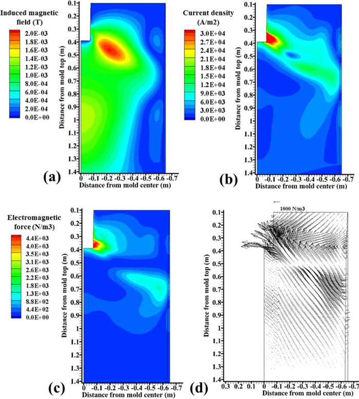
In the mold region, the induced magnetic field, induced current density, and Lorentz force are presented in Fig. 5 for the case with the realistic steel shell. High Lorentz forces are observed in two regions corresponding to high current density: near the nozzle port and near the NF 600 mm below the mold top. The direction of the force opposes the flow of the jet, which agrees with theory. While also retaining mass and momentum balances, the result is deflection of the jet flow away from these two regions. For the conditions here, the easiest path for jet deflection is downward, towards the lower strand where the magnetic field is weaker, especially near the NF.

Fig. 5.

(a) Induced magnetic field, (b) current density, (c) electromagnetic field, and (d) electromagnetic force vector distributions in the mold. (Online version in color.)

4.2. EMBr Effect on Nozzle Flow

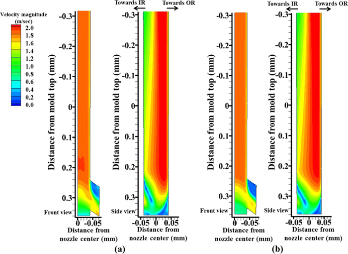
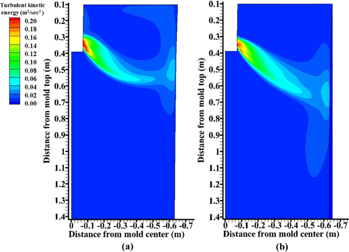
As shown in Fig. 6, the EMBr effect on the mean nozzle flow is small, even though the Lorentz force in the nozzle is strong. Predicted velocity contours without and with EMBr are very similar at these two center-plane cross sections (front and side views). The clockwise-rotating swirl flow produced by asymmetric opening area of the middle plate of the slide-gate¹⁸⁾ exists both without and with the EMBr. However, the EMBr significantly affects the velocity fluctuations in the nozzle. As shown in Fig. 7, EMBr decreases the turbulent kinetic energy considerably at the well-bottom region, especially in the side-center view. This means that the rotating flow experiences fewer variations and changes in direction with EMBr.

Fig. 6.

Predicted velocity magnitude in the nozzle (a) without EMBr and (b) with EMBr. (Online version in color.)

Fig. 7.

Turbulent kinetic energy in the nozzle (a) without EMBr and (b) with EMBr. (Online version in color.)

4.3. EMBr Effect on Mold Flow

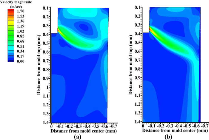
Velocity contours in the mold are compared in Fig. 8. Without EMBr, the jet impinges high on the NF wall, induces strong flow upward along the NF, and results in high surface velocity. The strong flow near the meniscus could be detrimental in shearing off and entraining slag at the surface. With EMBr, however, jet flow in the mold is deflected downward by the strong Lorentz forces induced in the regions near the ports, and near the NF, 600 mm below mold top. This produces a steeper downward angle of impingement on the NF, with less flow up the NF and consequently slower surface velocity. The strong downward mean flow along the NF with EMBr could be undesirable by taking argon bubbles and inclusions deep into the mold cavity, resulting in more internal defects. The jet flow is expected to have smaller turbulent kinetic energy with EMBr, especially towards the top surface, as shown in Fig. 9. On the other hand, turbulent kinetic energy increases below the jet impingement point with EMBr, indicating more detrimental velocity variations in the lower strand. This finding differs from that of previous researchers,^14,17) where both surface flow and downward flow greatly decrease with double-ruler EMBr. This is likely because the fields and casting conditions were different. Perhaps of greatest significance, the magnetic fields of these previous studies were uniform across the mold width, which contrasts with the present measured fields, which decreased greatly towards the NF.

Fig. 8.

Predicted velocity magnitude on center-middle plane in the mold (a) without EMBr and (b) with EMBr including steel shell. (Online version in color.)

Fig. 9.

Turbulent kinetic energy predicted in mold mid-plane (a) without EMBr and (b) with EMBr including steel shell. (Online version in color.)

5. Model Validation

The predicted profiles of surface level, velocity magnitude and their fluctuations across the mold surface are compared with measurements from a series of nail-board dipping tests in Figs. 10 and 11, both with and without EMBr. For both conditions, ten nail-board tests were taken during 9 minutes in the 2010 trial at both the Inside Radius (IR) and Outside Radius (OR), and averaged both temporally and spatially. The measurements without EMBr were shown in Part I.¹⁸⁾ The measurements with EMBr (DC 300A to both rulers) are presented in Section 6. Both sets of measurements are compared here with model predictions along the center line of the top surface. In addition to the best predictions using the realistic solid shell, model predictions are also presented with perfectly-conducting and perfectly-insulated walls for comparison purposes.

Fig. 10.

EMBR effect on (a) time-averaged surface level profile and (b) surface level fluctuations. (Online version in color.)

Fig. 11.

EMBR effect on (a) time-averaged surface velocity and (b) surface velocity fluctuations. (Online version in color.)

The surface level profile was calculated from the surface pressure with Eqn 23 in Part I.¹⁸⁾ The surface level fluctuation Δh was estimated from the turbulent kinetic energy k predicted by the standard k–ε model as follows.¹⁹⁾   

$$\mathrm{\Delta }\mathrm{h}=\frac{\mathrm{k}}{\mathrm{g}}$$(4)

where g is gravity acceleration. Similar to the assumption for surface level, slag density is not considered in Eq. (4) because measurements presented here in Section 6 show that the slag is lifted more than it is displaced. Huang and Thomas found that surface level fluctuations predicted from Eqn 4 matched well with measurements.¹⁹⁾ Surface velocity fluctuations $\overline{\left|{{\mathrm{u}}^{\prime }}_{\mathrm{i}}\right|}$ were calculated from the turbulent kinetic energy k by assuming that components in the 3 coordinate directions (i) are isotopic.   

$$\overline{\left|{{\mathrm{u}}^{\prime }}_{\mathrm{i}}\right|}=\sqrt{\frac{2}{3}\mathrm{k}}$$(5)

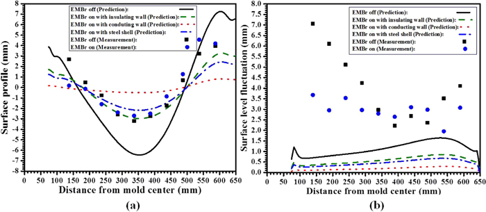
The surface level is flatter with EMBr, in both the predictions and the measurements, as shown in Fig. 10(a). The surface level is highest near the NF, and lowest at the quarter point in both predictions and measurements, as found in previous work.^8,9,15,16) The predicted level is much flatter with EMBr, but the measured level profile variations decrease only near the SEN. The best prediction with the realistic steel shell matches well with the measurements with EMBr. Without EMBr, however, the predictions significantly over-predict the extent of the variation in surface level profile across the width.

Surface level fluctuations decrease with EMBr in both the predictions and the measurements, but the magnitudes and variations differ, as shown in Fig. 10(b). The predicted fluctuations are much smaller than the measurements, are smallest near the SEN, and decrease with EMBr along the entire surface. One the other hand, the measured fluctuations are much larger near the SEN and NF, likely due to sloshing waves, which are not possible to capture with the current model. Furthermore, the measured fluctuations decrease only from the quarter point to the SEN. Thus, the model Eq. (4) is very crude and gives only a very rough estimate of level fluctuations.

Surface velocity decreases with EMBr, in both the predictions and the measurements, as shown in Fig. 11(a). Surface velocity is a maximum at the quarter point, and decreases towards the SEN and NF. This trend and quantitative predictions with the realistic steel shell match well with the measurements with EMBr. The extent of the reduction of surface velocity caused by EMBr is over-predicted, however. The model predicts 43% reduction, but the measurements show only 17% reduction.

Surface velocity fluctuations with EMBr also decrease in both the predictions and the measurements, as shown in Fig. 11(b). The model predictions again match well with the measurements with EMBr. However, the extent of the reduction with EMBr is slightly under-predicted. The model predicts 37% reduction, but the measurement shows 43% reduction.

The discrepancy in the model predictions without EMBr is likely due to the neglect of argon gas injection. It seems that 5.6% argon gas volume injected in the real caster is not negligible, and has an important effect on the flow pattern and surface behavior, especially without EMBr. Future models should incorporate these multiphase flow effects. Further model improvements are also needed to make better predictions of transient phenomena, such as using LES models, and to incorporate gravity wave effects, such as using a free–surface model. Nevertheless, the simple model used here when considered together with the measurements provides important insights into understanding the effect of EMBr on nozzle, mold, and surface flow behavior.

Finally, the predictions with three different wall conductivity conditions (perfectly-conducting wall, -insulating wall, and realistic solid shell) are compared in Figs. 10 and 11. The predictions of surface phenomena with the realistic solid shell fall between the less-appropriate cases of perfectly-insulating and -conducting walls.

6. Measurement Results

The effect of EMBr on surface level and surface velocity is quantified by measurements using an eddy-current sensor and nail board dipping tests in plant experiments conducted in 2008 and 2010 and explained in Part I.¹⁸⁾

6.1. Surface Level (2010 Trial)

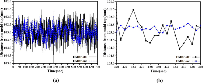
The transient time-history of surface level of the molten steel was measured by a standard commercial eddy current sensor at the “quarter point” located midway between the SEN and the NF both with and without EMBr. Signals were collected with 1 sec moving time averaging for 700 sec, as shown in Fig. 12(a). Replotting of a 20 sec interval with expanded scale in Fig. 12(b) shows the multiple frequencies of the level rises and drops. The average surface level is ~103 mm for both cases. The amplitude of the level variations is clearly greatly lowered with EMBr, as expected. Specifically, the level fluctuations drop from ~0.6 mm without EMBr to ~0.4 mm with EMBr.

Fig. 12.

Surface level variations measured by the eddy current sensor during (a) 700 sec and (b) 20 sec with expanded scale. (Online version in color.)

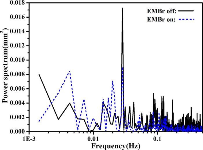
Power spectrum analysis of the eddy-current surface level in Fig. 12 is shown in Fig. 13. Due to the data collection time interval of 1 sec, and total collection time of 700 sec, frequencies could be calculated only in the range from 0.5 Hz to 0.0014 Hz. A very strong maximum peak is observed at ~0.03 Hz, both with and without EMBr, which corresponds to periodic flow oscillations of ~35 sec. Without EMBr, many periodic level fluctuations are observed, including a peak at ~0.1 Hz for asymmetric flow past the SEN predicted using Honeyands and Herbertson’s relation.²⁰⁾ With EMBr, the power of this maximum peak is decreased by ~50% and other peaks in the power spectrum at frequencies > ~0.03 Hz, are decreased significantly with EMBr. Thus, EMBr stabilizes the surface level by dampening the fluctuations with higher frequencies > ~0.03 Hz.

Fig. 13.

Power spectrum of the surface level signal measured by the eddy current sensor. (Online version in color.)

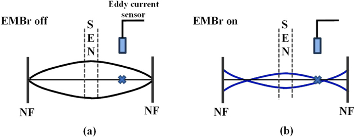
To investigate the effect of EMBr on the surface level at other regions of the mold surface, the transient surface level profiles of the molten steel and the slag were measured by 10 nail board dipping tests taken over 9 minutes both with and without EMBr. As shown in Fig. 14, both conditions show evidence of sloshing, where the level is alternatively higher and then lower near the SEN and near the NF. The steel level measured by the eddy current sensor is shown as a cross symbol, located at its actual position near the quarter point on the opposite side of the mold. The level at this location matches the nail board measurements well, which shows that the measurements on opposite sides of the mold are consistent and symmetrical. More significant is that the level at the eddy-current sensor location varies very little during this time, while the SEN and NF fluctuate greatly. This finding suggests that the eddy current sensor was positioned near a central “node” which best indicates the average level, and enables the level control system to maintain a stable average molten steel level. However, this finding confirms that the sensor is unable to detect the large level variations at other regions of the mold surface, such as due to sloshing. Furthermore, it should not be designed to detect them. The time-averaging of the sensor signal is another means that the sensor signal is stabilized and another reason that the large level variations are missed.

Fig. 14.

Transient variations of surface level profile (a) without and (b) with EMBr by the nail board measurements. (Online version in color.)

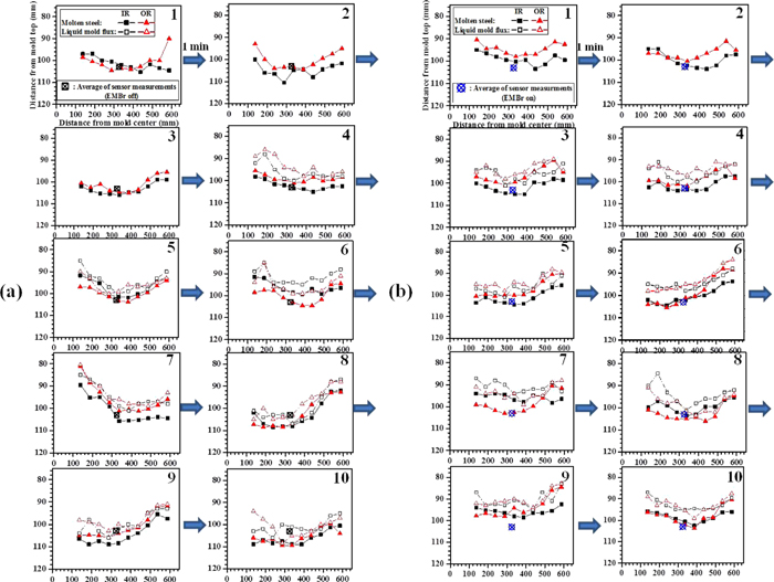
The time-averaged surface level with EMBr was slightly (~3 mm) higher than without EMBr, as shown in Fig. 15(a). This effective change in the level set-point is inconsequential to quality, although it is interesting that this difference was not detected by the eddy-current sensor. This likely indicates variations in average level between the two sides of the mold.

Fig. 15.

EMBR effect on (a) time-averaged surface level and (b) surface level fluctuation by the nail board measurements. (Online version in color.)

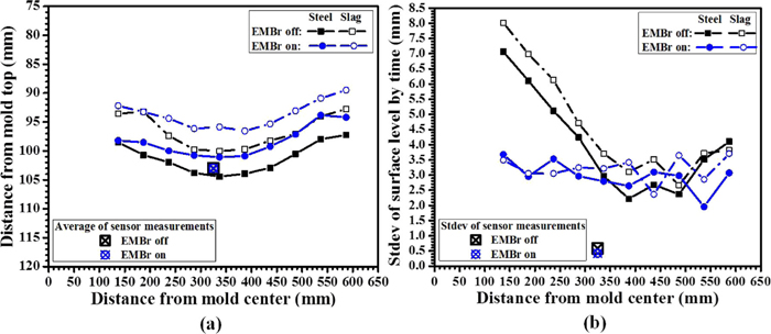
The level fluctuations, as indicated by the standard deviation (stdev) of the level measurements, are greatly decreased with EMBr, especially near the SEN, as shown in Fig. 15(b). Without EMBr, level fluctuations become severe towards the SEN, showing maximum average fluctuations of over 7 mm. On the other hand, with EMBr, the maximum average fluctuations are decreased to < 4 mm, and are more uniform across the mold width (average ~3.3 mm). Average level fluctuations across the mold width are ~4.0 mm without EMBr and ~3.0 mm with EMBr. The lowest fluctuations are found near the quarter point without EMBr and slightly off the quarter point with EMBr. This trend appears due to the sloshing mechanism, which is explained in the next section.

6.2. Surface Level and Sloshing (2008 Trial)

The transient time-history of surface level was measured with 6 nail board tests over 5 minutes in the 2008 trial under the same casting conditions as the 2010 trial in Fig. 14, with and without EMBr. The surface levels at each location across the mold width, were averaged over inside and outside radius, and all plotted together in Fig. 16. As in the 2010 trial, large periodic variations are observed both with and without EMBr, showing sloshing behavior. During the 5 minutes, the surface level shows at least two periodic oscillations without EMBr, and at least three with EMBr. Considering the peak at 35 sec in the 2010 trial, the 6 snapshots measured in 2008 may have been taken over as many as 9 major oscillations in surface level.

Fig. 16.

Measured molten steel surface level shape (a) without EMBr and (b) with EMBr. (Online version in color.)

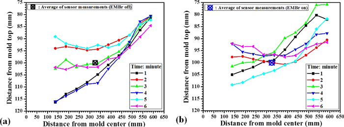
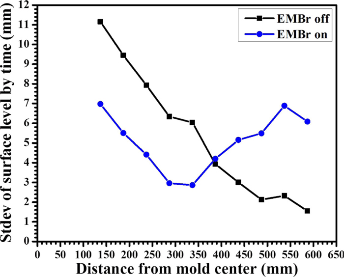
The set-point (target) level for the eddy current sensor, shown as a cross-symbol, again shows significantly more stability at its quarter point location than the rest of the mold surface. The level variations are generally less with EMBr, both at this location, and across the mold width. The greatest fluctuations are found near the SEN without EMBr, as shown in Fig. 16 (maximum difference > 25 mm) and Fig. 17 (standard deviation > 11 mm). With EMBr, the fluctuations decrease to only 7 mm near the SEN, but increase to 6 mm near the NF, where they were < 2 mm without EMBr.

Fig. 17.

Measured molten steel surface level fluctuations without and with EMBr. (Online version in color.)

A wave sloshing mechanism to explain the level variation behavior in 2008 is illustrated in Fig. 18. Decreasing fluctuations observed from the SEN towards the NF without EMBr are consistent with the oscillating wave shape shown in Fig. 18(a). Minimum fluctuations at the quarter point, observed with EMBr, are consistent with the waves in Fig. 18(b). Although this mechanism does not exactly match all of the 2010 trial measurements, it is consistent with the improvement in level stability with EMBr recorded at the quarter point by the eddy-current sensor (on average and at the 0.03 Hz peak), and with the lack of improvement at the NF nails. Thus, the eddy-current sensor should be positioned near stable nodes in the surface waves if possible, and the large detrimental sloshing variations should be measured independently, using nail boards tests.

Fig. 18.

Schematic of the sloshing level mechanism (a) without and (b) with EMBr. (Online version in color.)

6.3. Slag Layer Behavior (2010 Trial)

Slag level profiles were also measured via the nail board experiments, as explained in Part I,¹⁸⁾ and show transient variations that correspond to the level variations of the molten steel. Sloshing of the slag level is observed both with and without EMBr in Figs. 14 and 15(a). The surface level profile of the slag/powder interface generally follows the rising and falling of the steel/slag interface. The difference between these slag and steel levels indicates the thickness of the liquid slag layer. The relative lack of thickness variations suggests that the slag layer is simply lifted up and down by the steel motion.

To further investigate this phenomenon, the slag level is plotted as a function of the steel level in Fig. 19. Both level heights are measured from the time average of the steel levels. Data were divided into three regions: SEN region 1 from 135 mm to 235 mm, Quarter-point region 2 from 235 mm to 485 mm, and NF region 3 from 485 mm to 585 mm from the mold center. Linear trend lines are plotted in each region, and included in Fig. 19. The coefficients of these linear equations have physical meanings. The constant (y-intercept) means average thickness of the liquid slag layer, and the slope quantifies the slag motion. A slope of 0 means that slag motion is totally caused by displacement of some liquid slag by molten steel, as gravity causes the slag to flow down to where the steel level profile is lower in order to accommodate a local rise in the steel level. A slope of 1 means that the slag level is simply lifted up and down by the steel level motion, with no change in thickness.

Fig. 19.

Relation between molten steel level and liquid mold flux level (a) without EMBr and (b) with EMBr by the nail board measurements. (Online version in color.)

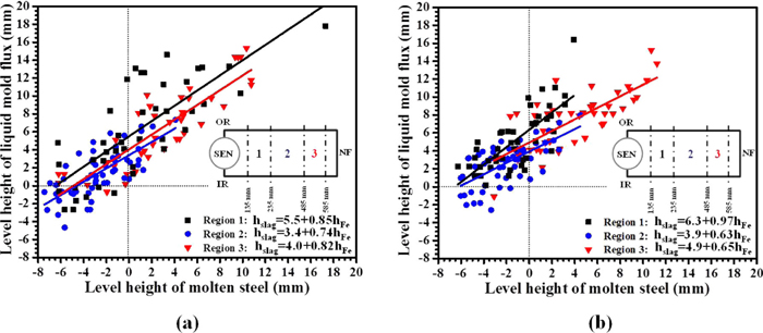
The slag behavior in SEN region 1 shows mainly lifting, especially with EMBr. The other regions show a significant (up to 37%) displacement component of motion, especially with EMBr. The slag thickness in all regions is slightly larger with EMBr. Perhaps this is because smaller level fluctuations lead to shallower average oscillation mark depth, decreasing slag consumption slightly, and thus allowing a slightly thicker slag layer to build up.

The thinnest slag layer is found in the quarter-point region 2, both with and without EMBr. Thomas et al. found that temperature of the molten steel is expected to be highest near the midway point of a double-roll flow pattern.^21,22) The finding here offers proof that higher steel temperature is not as effective as convective mixing due to steel flow in controlling the melting behavior of the slag and the slag layer thickness. Convection mixing inside the slag layer transports more heat to the powder and thereby increases melting rate and slag layer thickness.²³⁾ This is also obvious via the theory that a few degrees of temperature variation across the surface is negligible relative to drop across slag layer over 1000°C, so should theoretically have negligible effect on slag melting. The mixing mechanism is likely enhanced by higher steel surface velocity, level fluctuations, and interaction with argon gas leaving the surface.

6.4. Surface Flow Pattern and Velocity (2010 Trial)

Transient flow patterns and velocity profiles across the molten steel surface were calculated from the 10 nail board dipping tests for 9 minutes both with and without EMBr, as shown in Figs. 20, 21, 22. The flow direction is given by a vector arrow with length proportional to the velocity magnitude. Flow is generally directed from the NF towards the SEN, according to a classic double-roll flow pattern. In addition, there is also a strong transient cross flow component, usually directed towards the inside radius, for both cases. Sometimes, the cross flow is towards the outside radius on one side, especially without EMBr. Very near the NF, surface flow goes slightly toward the NF, but is weaker with EMBr, suggesting there is less subsurface recirculating flow there with EMBr.

Fig. 20.

Transient variations of surface flow pattern (a) without and (b) with EMBr by the nail board measurements. (Online version in color.)

Fig. 21.

Averaged surface flow pattern (a) without and (b) with EMBR by the nail board measurements. (Online version in color.)

Fig. 22.

EMBR effect on (a) time-averaged surface velocity and (b) surface velocity fluctuation by the nail board measurement. (Online version in color.)

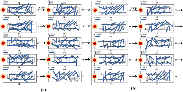
Average surface velocity profiles across the mold width are compared in Fig. 22(a). The classic profile with maximum velocity near the quarter point is found both with and without EMBr, and have similar magnitudes. The highest average surface velocity magnitude is found near the outside radius for both cases. On average, surface flow is slightly slower (by ~17%) with EMBr. Surface velocity fluctuations, as indicated by the standard deviation (stdev) of the velocity measurements, are smaller (by ~43%) with EMBr, as shown in Fig. 22(b). This finding suggests that use of the double-ruler EMBr for the conditions of this study may help to reduce defects caused by surface flow instability.

7. Conclusions

The effect of double-ruler EMBr on transient flow during steady continuous casting was investigated by applying a standard k–ε RANS model coupled with MHD equations and plant measurements using an eddy-current sensor and nail boards.

• The double-ruler “FC-Mold” EMBr studied here creates two regions of equally-strong magnetic field across the mold width: one centered just above the port and the other centered farther below the nozzle port. Both peaks in the measured field significantly decrease in strength towards the NF.

• With EMBr, turbulent kinetic energy is decreased in the nozzle well region, where rotating swirl flow is caused by the asymmetric open area at the slide-gate.

• Jet flow with this EMBr configuration is deflected downward, resulting in flatter surface level and slower surface velocity with less fluctuations.

• With EMBr, the predicted surface level profile, velocity profile, surface level fluctuations, and velocity fluctuations all match surprisingly well with the measurements, considering the simplified model. Without EMBr, the model over-predicts the level profile variations and the surface velocities, and underpredicts the fluctuations.

• The surface level fluctuations measured by an eddy-current sensor of 0.6 mm (Without EMBr) and 0.4 mm (With EMBr) are much smaller than those by the nail board dipping tests, of 4.0 mm (Without EMBr) and 3.0 mm (With EMBr). This is likely because the eddy-current sensor is positioned over a near-stationary node in the waves, and its signals are filtered (1 sec time-average) according to standard industry practice, to miss the real transient fluctuations which are captured by the nail board tests.

• Both with and without EMBr, the surface level experiences periodic variations which show sloshing between the SEN and the NF, as indicated by sequences of nail board dipping tests. The sloshing is high amplitude (up to 8 mm) and low frequency / long period (up to 1 minute).

• Both with and without EMBr, a characteristic frequency peak of the surface level variations is observed at ~0.03 Hz (~35 sec) at the “quarter point” located midway between the SEN and the NF.

• EMBr increases surface level stability, specifically by decreasing the severe level fluctuations near the SEN by ~50%, and lowering the peaks in the level fluctuation power spectrum.

• Motion of the steel-slag interface level mainly causes lifting of the slag layers, especially near the SEN. Elsewhere, the slag layers are partially displaced by the steel, due to flow that causes the liquid layer to become slightly thinner, especially near the NF, and with EMBr.

• The slag pool is slightly thicker with EMBr.

• The surface flow with EMBr shows more biased cross-flow pattern from outside to inside radius.

• EMBr produced ~20% lower surface velocities (Without EMBr: 0.22 m/sec, With EMBr: 0.18 m/sec) with ~40% less velocity variations (Without EMBr: 0.12 m/sec, With EMBr: 0.07 m/sec).

• Double-ruler EMBr may help to reduce defects caused by surface instability if used properly.

Acknowledgements

The authors thank POSCO for their assistance in collecting plant data and financial support (Grant No. 4.0004977.01), and Mr. Yong-Jin Kim, POSCO for help with the plant measurements. Support from the National Science Foundation (Grant No. CMMI 11-30882) and the Continuous Casting Consortium, University of Illinois at Urbana-Champaign, USA is also acknowledged.

References

• 1)   K.  Takatani,  K.  Nakai,  T.  Watanabe and  H.  Nakajima: ISIJ Int., 29 (1989), 1063.
• 2)   K.  Moon,  H.  Shin,  B.  Kim,  J.  Chung,  Y.  Hwang and  J.  Yoon: ISIJ Int., 36 (1996), S201.
• 3)   Y.  Hwang,  P.  Cha,  H.  Nam,  K.  Moon and  J.  Yoon: ISIJ Int., 37 (1997), 659.
• 4)   H.  Harada,  T.  Toh,  T.  Ishii,  K.  Kaneko and  E.  Takeuchi: ISIJ Int., 41 (2001), 1236.
• 5)   B.  Li and  F.  Tsukihashi: ISIJ Int., 43 (2003), 923.
• 6)   Z.  Qian and  Y.  Wu: ISIJ Int., 44 (2004), 100.
• 7)   H.  Yu and  M.  Zhu: ISIJ Int., 48 (2008), 584.
• 8)   K.  Cukierski and  B. G.  Thomas: Metall. Mater. Trans. B, 39B (2008), 94.
• 9)   Y.  Wang and  L.  Zhang: Metall. Mater. Trans. B, 42B (2011), 1319.
• 10)   B.  Li,  T.  Okane and  T.  Umeda: Metall. Mater. Trans. B, 31B (2000), 1491.
• 11)   B.  Li,  T.  Okane and  T.  Umeda: Metall. Mater. Trans. B, 32B (2001), 1053.
• 12)   K.  Timmel,  S.  Eckert,  G.  Gerbeth,  F.  Stefani and  T.  Wondrak: ISIJ Int., 50 (2010), 1134.
• 13)   K.  Timmel,  S.  Eckert and  G.  Gerbeth: Metall. Mater. Trans. B, 42B (2011), 68.
• 14)   R.  Chaudhary,  B. G.  Thomas and  S. P.  Vanka: Metall. Mater. Trans. B, 43B (2012), 532.
• 15)   R.  Singh,  B. G.  Thomas and  S. P.  Vanka: Metall. Mater. Trans. B, in press.
• 16)   S.  Cho,  H.  Lee,  S.  Kim,  R.  Chaudhary,  B. G.  Thomas,  D.  Lee,  Y.  Kim,  W.  Choi,  S.  Kim and  H.  Kim: Proc. of TMS2011, TMS, Warrendale, PA, USA, (2011), 59.
• 17)   R.  Singh,  B. G.  Thomas and  S. P.  Vanka: CCC Report 201302, University of Illinois, Ill, (2013).
• 18)   S-M.  Cho,  S-H.  Kim and  B. G.  Thomas: ISIJ Int., 54 (2014), 845.
• 19)   X.  Huang and  B.  Thomas: Can. Metall. Q., 37 (1998), 197.
• 20)   T. A.  Honeyands and  J.  Herbertson: 127th ISIJ Meeting, ISIJ, Tokyo, (1994).
• 21)   B. G.  Thomas,  F. M.  Najjar and  L. J.  Mika: Proc. of Weinberg Symp. on Solidification Proc., CIM, Canada, (1990), 131.
• 22)   X.  Huang,  B. G.  Thomas and  F. M.  Najjar: Metall. Mater. Trans. B, 23B (1992), 339.
• 23)   B.  Zhao,  S. P.  Vanka and  B. G.  Thomas: Int. J. Heat Fluid Fl., 26 (2005), 105.