Thermo-mechanically Coupled Isotropic Analysis of Temperatures and Stresses in Cooling of Coils

Abstract

A 2D transient thermo-mechanically coupled axi-symmetric FE model has been implemented and used to predict the temperatures and stresses under cooling of coils. The temperature trajectory as a function of geometrical position in as-coiled steel strip products is affected by several parameters as the: initial temperature inherited from upstream cooling on the Run Out Table (ROT), coil dimensions, strip surface quality, contact conditions and the surrounding environmental conditions etc. The layered structure makes the thermal conductivity anisotropic where the interfacial contact condition depends on the transient stress state caused by thermal and initial effects. The coil cooling rates are for HSLA-steel grades of importance in achieving proper final mechanical properties where too fast temperature drops ceases the precipitation hardening solely diffusional driven. Furthermore is a parameter influence study made revealing process parameter significance. The model has been validated against two full-scale bell furnace trials. A main objective with this model development work was to keep the model fast and accurate applicable on real plant situation and for process controlling.

1. Introduction

Hot rolled strips that can obtain lengths between 200–2000 m are winded up in a coil after being hot rolled and cooled at the run out table. The coil immediately starts to cool from the initial temperature of approximate 600–700°C (depending on grade) to a steady state condition at room temperature which takes several days. The thermal conductivity exhibits strong anisotropy in radial and axial directions respectively due to the layered structure including interfacial contact zones. The interfacial or gap conductivity in radial direction depends on surface conditions, strip shape, coiler settings and contact pressures (radial stresses). The radial stresses are initially set by the coiling process^1,2,3) but during cooling thermal stresses will be superposed to the initial stress state. At the boundary laps the lower radial stresses results in a faster temperature drop due to reduced radial heat transfer from core parts. Thus for some grades e.g. HSLA (High Strength Low Alloy) steels this reduces diffusion of alloying elements and thereby a limitation in the precipitation hardening.⁴⁾ To predict the transient temperature distribution in the coils in this study a 2D thermo-mechanical axi-symmetric Finite Element (FE) model was implemented. This work is an extension of a previous study^4,5) by addition of a structural solution to include transient contact pressure dependent thermal conductive properties.

The model accounts for the imperfect and pressure dependent contact conditions between adjacent laps causing anisotropies in thermal properties. The interfacial strip, surface-to-surface contact is in a macroscopic level dependent on oxide, dust, water and strip shape properties inherited from up-stream processes and in a microscopic level by surface conditions like roughness and slope of asperities etc. This model uses an equivalent unit contact conductance concept to model the interfacial zones on a continuum.^{1,5,6,7,8,9,10,11)} Commonly previous investigations have based their contact formulation on previous work performed by Mikic et al.¹²⁾ The current work is based on a model by Shridar et al.¹³⁾ including micro elasto-plastic deformation effects of the surface asperities. The stresses have an influence on the contact conditions and can be subdivided into initial stresses set by the coiler and the thermally induced stresses. Initial stress conditions are set by strip geometric properties and coiler settings.^1,3,5,8,10) In the previous model⁵⁾ a constant radial pressure function to calculate gap zone properties was used, with good predictability but process variations in pressure due to strip shape, coiler settings and quality etc. was not able to be captured. An approximation that made the model static in both radial and axial directions and too generalized for real processes and further predictions of e.g. mechanical properties. Compared to previous models^{1,2,3,4,5,6,7,8,9,10)} an elastic-plastic contact approach¹²⁾ is used and the initial stresses are calculated non-linearly in 2D. Furthermore is the coupled thermo-mechanical problem solved by use of FEM rather than FD or commercial FEM softwares which makes this model perfectly suitable for in or on-line applications, or part of a process control optimization system but with no loss in accuracy.

2. Models and Numerical Implementation

2.1. Thermal Model

The thermal model used in this paper is in detail described elsewhere⁵⁾ and is therefore only briefly described below. The axi-symmetric FE model domain is displayed in Fig. 1.

Fig. 1.

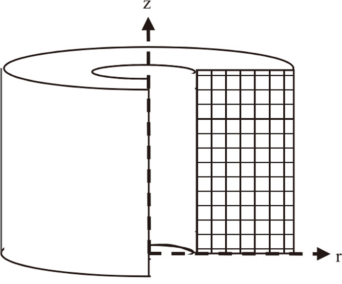
Spatial discretization of the FEM model.

The Fourier non-linear heat conduction equation in cylindrical coordinates is used and written as   

$$\frac{1}{r}\frac{\partial }{\partial r}\left({\kappa }_r\left({\sigma }_r\right)\cdot r\cdot \frac{\partial T}{\partial r}\right)+{\kappa }_z\frac{{\partial }^{2}T}{\partial z^2}=\rho C_p\frac{\partial T}{\partial t}$$(1)

Where T is the temperature, κ_r and κ_z are the thermal conductivity in the spatial directions, ρ is the density and C_p the specific heat capacity. With the boundary conditions applied on the inner and outer boundaries resp.   

$$\begin{array}{l}{\kappa }_r\cdot \frac{\partial T}{\partial r}=q_r+q_c,\mathrm{\hspace{0.17em} }{\kappa }_z\cdot \frac{\partial T}{\partial r}=q_r+q_c\mathrm{\hspace{0.17em} }\text{and}\\ -{\kappa }_r\cdot \frac{\partial T}{\partial r}=q_r+q_c,\mathrm{\hspace{0.17em} }\mathrm{\hspace{0.17em} }-{\kappa }_z\cdot \frac{\partial T}{\partial r}=q_r+q_c\end{array}$$(2)

The initial conditions are   

$$T_0=T$$(3)

The initial temperature T₀ used in the modelling is a result of the cooling at the ROT section. Finite element semi-discretisation of the thermal problem leads to system of coupled nonlinear equations.   

$${\mathbf{K}}_{th}\cdot \mathbf{T}+\mathbf{C}\cdot \dot{\mathbf{T}}={\mathbf{F}}_{th}$$(4)

K_th and C are the conductance and capacitance matrices resp. and F_th is the consistent load vector. The implicit Backward Euler Finite difference scheme is used for the time stepping. This leads to a nonlinear system of coupled equations that is solved by the Newton-Raphson method.¹⁴⁾ The outward boundary conditions are nonlinear and heat transfer takes place by radiation and natural convection.^5,15,16,19) At the outward boundary the radiation view factor equals one but is at the inward surface a function of geometries of the coil.⁵⁾

2.2. Thermal Properties

The thermal conductivity in axial direction is similar to the conductivity of the steel⁵⁾ whereas in radial direction it accommodates the layered structure of the coil. The layered structure makes this problem anisotropic where thermal conductivities in radial directions must account for contact zone properties schematically displayed in Fig. 2 as thermal resistances over one contact zone. The heat transfer over the gap zone occurs by convection, radiation and conduction, the latter one is dominant according to Kraus et al.¹⁷⁾ whereas the two other ones are neglected.

Fig. 2.

Schematic description of the thermal contact situation of one unit coiled material. The dashed squares are neglected.

This is modelled by calculating element wise equivalent radial thermal conductivities based on the thicknesses and thermal conductivities of the contact zone, oxide scale and steel strip respectively.^4,5,6,7,8,9) The radial equivalent thermal conductivity can be, via the thermal resistance, be written as   

$$R=R_{steel}+2R_{oxide}+R_{gap}\Rightarrow \frac{t_{tot}}{{\kappa }_{eq}}=\frac{t_{steel}}{{\kappa }_{steel}}+2\cdot \frac{t_{oxide}}{{\kappa }_{oxide}}+\frac{t_{gap}}{{\kappa }_{gap}}$$

  

$$\begin{array}{l}{\kappa }_{eq,i}^{}=\\ \frac{\left(t_{steel}+2t_{oxide}+t_{gap}({\sigma }_r)\right)\cdot {\kappa }_{steel}{\kappa }_{oxide}{\kappa }_{gap}({\sigma }_r)}{\left(t_{gap}({\sigma }_r){\kappa }_{steel}{\kappa }_{oxide}+t_{steel}{\kappa }_{oxide}{\kappa }_{gap}({\sigma }_r)+2t_{oxide}{\kappa }_{steel}{\kappa }_{gap}({\sigma }_r)\right)}\\ i=1\dots n,n=\text{number of el}.\end{array}$$(5)

κ_steel, κ_oxide and κ_gap are the thermal conductivities for each component with corresponding thicknesses t_steel, t_oxide and t_gap. The equivalent thermal conductivity, κ_eq is approximated as constant in each element. Note, in previous work,⁵⁾ Eq. (5) was incorrectly missing a factor 2 in the numerator. The thermal conductivity for oxide has been investigated by e.g. Park et al.⁶⁾ and was reported to be approximately 3 W/mK and to be ca 7–10 μm thick. The model by Shridar et al.¹³⁾ has been used in the current work for the thermal properties of the gap zone i.e. κ_gap and t_gap. These properties are functions of the radial stress state.

2.3. Coil Winding, Initial Stress State Model

The moment in the coiler generates a tension in the strip under coiling. This tension together with the strip thickness variation across the width is essential parameters for predicting the initial stress state in the coil. In steel strip production the hot strip to be coiled is almost always carrying a mid-thick profile that accumulates into a “barrel” shape causing decreased/increased compressive stresses in edges and mid-section respectively.

By assuming that no interfacial sliding occurs between individual laps²⁾ the coil can be approximated as a continuum whereas, the problem can be approximated as a linear elastic boundary value problem,¹⁸⁾ see Fig. 3. Since neither strip bending nor stress and strain variations are encountered for across the strip thickness the model stresses/strains becomes constant on a cross section in length direction and consequently no plastic deformations are present due to the low effective stress levels.

Fig. 3.

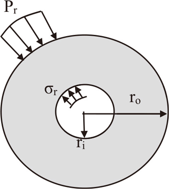
Geometrical domain and boundary conditions to the analytical boundary value problem.

The general solution of the radial displacements is   

$$u_r(r)=A_1\cdot r+\frac{A_2}{r}\mathrm{\hspace{0.17em} }\mathrm{\hspace{0.17em} }\text{where}\mathrm{\hspace{0.17em} }\mathrm{\hspace{0.17em} }{\epsilon }_r=\frac{d{u}_r}{dr},{\epsilon }_{\phi }=\frac{u_r}{r}$$(6)

A₁ and A₂ are integration constants, r is the radius and u_r the radial deformation. An isotropic linear elastic approach gives according to Hooke’s law   

$${\sigma }_r(r)=\frac{E}{1-{\upsilon }^2}\cdot \left(A_1\cdot (1+\upsilon )-A_2\cdot (1-\upsilon )\cdot \frac{1}{r^2}\right)$$(7)

  

$${\sigma }_{\phi }(r)=\frac{E}{1-{\upsilon }^2}\cdot \left(A_1\cdot (1+\upsilon )+A_2\cdot (1-\upsilon )\cdot \frac{1}{r^2}\right)$$(8)

where E is the Young’s modulus, σ_r, the radial- and σ_φ circumferential stresses and υ the Poisson’s ratio.

The geometry is expanded with a new ring for every lap. The coiler tension then becomes the circumferential stress at the n:th lap which is transferred to a compressive stress acting on the first to the n-1 layer. The following boundary conditions are applied for every new lap   

$${\sigma }_r(r_i)=0\mathrm{\hspace{0.17em} }\mathrm{\hspace{0.17em} }\text{and}\mathrm{\hspace{0.17em} }\mathrm{\hspace{0.17em} }{P}_r(r_o)=\frac{{\sigma }_{\phi }\cdot t}{r}$$(9)

where P_r is the pressure, t is the strip thickness, r the radius where inward and outward radius is indexed by i and o resp. The inner boundary condition implicates that displacement of the inner surface not is prescribed i.e. mandrel is never considered to be present. The external pressure boundary condition must be solved iteratively for each lap until the stress and the radial deformations are balanced where the stress boundary condition is updated via.   

$${\sigma }_{\phi }=E\cdot ln\left(\frac{r}{r_0}\right)$$(10)

where r₀ is the current “stress free” radius of the last coiled lap. After every added lap a converged stress state is found and accumulated to the previous ones.

In z-direction (across the strip) the model is subdivided into a discrete set of fibers to include effects of the strip thickness profile. The stress in each fiber is solved independent of the other fibers. An approximate formula for strip thickness profile^2,5,18) is for simplicity used.   

$$t(z)=t_0\cdot \left(1-\alpha {\left(\frac{\left|z\right|}{h}\right)}^n\right)\mathrm{\hspace{0.17em} }\mathrm{\hspace{0.17em} }0\le z\le h$$(11)

The parameters t₀ and t are the center and the strip thickness respectively, α is the strip crown ratio, n is the strip crown shape, h is the half strip width and z the width coordinate from strip center. For an investigated set of hot rolled strips, typical values on α and n are in the range 0.01–0.035 and 2–6 respectively. The strip profile causes an inhomogeneous stress distribution in the z-direction but there exist no constitutive direct coupling between the fibers in the model. Due to the accumulation of these profile effects, tensile stresses that eventually arise according to the linear elastic isotropic material approach are set to zero during the iterations. In Fig. 4, the influence of the strip profile parameters α, n and the coiler tension σ_T on the radial initial stresses solution in an as-coiled coil is depicted.

Fig. 4.

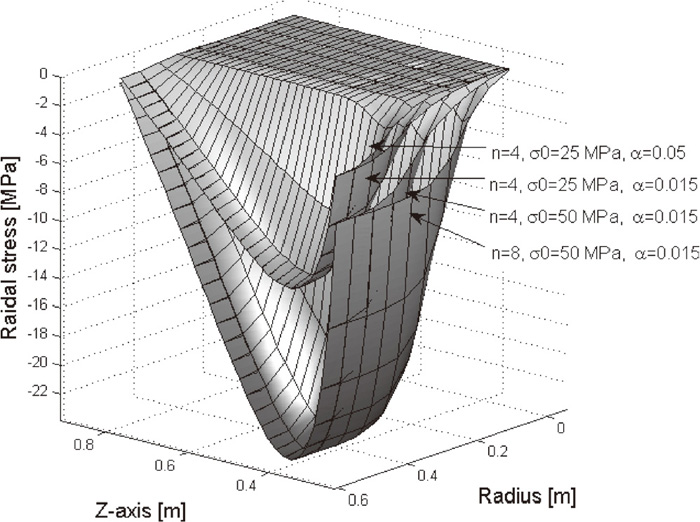
Influence of coil tension and profile parameters on the initial radial stress.

The coiler tension affects the radial stress magnitude meanwhile α and n mainly influences the shape of the stress profile caused by the accumulated strip shape.

2.4. Thermo-mechanically Coupled Solution

The thermal conductivities depend on the radial stresses in the coil due to coiling and the thermal stresses developing during cooling. Thus the thermal problem also requires a solution of the mechanical problem. The structural problem is solved by use of the same spatial discretization as for the thermal model where quadratic 4 node elements were used. The resulting semi-discretized equation of the structural FEM formulation becomes   

$$K\cdot U=F$$(12)

Where K is the stiffness matrix, U the nodal displacements and F the externally applied loads. Gravitational loads are ignored and the externally applied forces are due to thermal gradients. The thermal strains and initial stresses, σ₀ i.e. stresses caused by the coil winding are incorporated as consistent external forces via evaluation of element forces f as   

$$\begin{array}{c}f=\underset{v}{\int }{B}^T\sigma dV=\int B^T({\sigma }_0+D\cdot {\epsilon }_{th})dV\\ =\int B^T\left({\sigma }_0+D\cdot \alpha \left(T^t-T_0\right)\right)dV\end{array}$$(13)

where T₀, is the initial temperature, α is the thermal expansion coefficient for the present steel, here approximated as constant equal to 11•10⁻⁶ (1/K). Note, that orthotropic effects on the Youngs modulus and the thermal expansion due to influence of the interfacial gap zones is omitted in this study. B^T is the transposed strain-displacement matrix and D is the linear isotropic constitutive material matrix. The element forces are assembled to the global forces F. The displacement and the total stresses caused by thermal effects are attained via.   

$${\sigma }_c={\sigma }_0+D\cdot {\left(B\cdot u-{\epsilon }_{th}\right)}_c$$(14)

The element stresses evaluated at each element centroid, σ_c.

3. Results

3.1. Thermal Model, Calibration and Validation

To validate the model, measurements from a previous campaign was reused⁵⁾ where thermocouples were mounted on and into two coils with 0.0017 m and 0.006 mm thick strip respectively. Both coils were delivered by SSAB EMEA works in Borlänge and reheated in a full-scale bell furnace up to app 700°C. Additional coil information is summarized in Table 1.

Table 1. Coil properties.

Coil ID	Thickness (m)	Dia. (m)	Width (m)	Strip Crown, α	Strip Crown shape, n	Coiler Tension (MPa)
1	0.0017	0.85	1.1	0.015	2	50
2	0.006	0.85	1.1	0.015	2	50

The boundary conditions were calibrated based on measurements on the 0.0017 m thick strip coil, comparisons for reference points, p1–8 positioned according to Fig. 5, are displayed in Figs. 7, 8, 9, 10. The second coil (0.006 m) was used for validation, comparisons for reference points, p1,3,5 positioned according to Fig. 6 are displayed in Figs. 11, 12, 13. The same strip profile parameters were used for both coils.

Fig. 5.

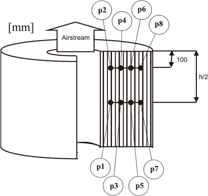
Measuring locations for the 0.0017 m coil.

Fig. 6.

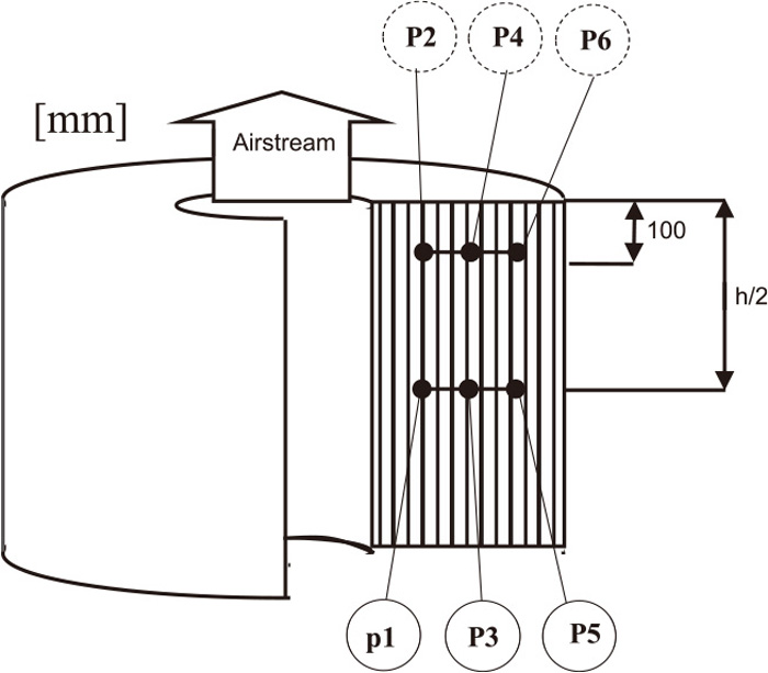
Measuring points for second coil, validation case. Dashed circles indicate fictive points used for evaluation of calculated stresses only.

Fig. 7.

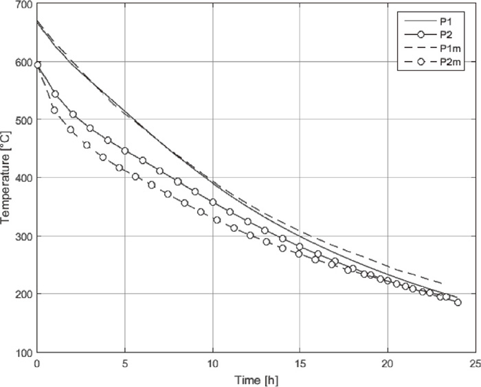
Comparison for reference point p1&2 located in r-direction 30 mm from inward surface.

Fig. 8.

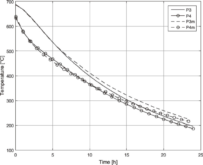
Comparison for reference point p3&4 located in r-direction 95 mm from inward surface.

Fig. 9.

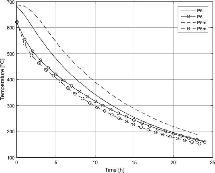
Comparison for reference point p5–6, 445 mm from inward surface.

Fig. 10.

Comparison for reference point p7–8, 525 mm and from inward surface.

Fig. 11.

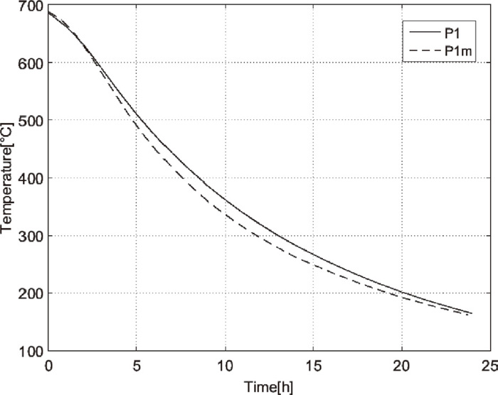
Comparison for reference point p1, 120 mm from inward surface.

Fig. 12.

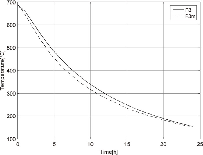
Comparison for reference point p3, 335 mm from inward surface.

Fig. 13.

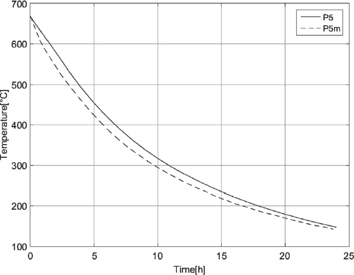
Comparison for reference point p5 120 mm from outward surface.

3.2. Stresses

Radial stresses are coupled to the thermal solution via the pressure dependent gap properties in Eq. (5). Figures 14, 15, 16, 17, 18 shows the calculated stresses for two different thicknesses at reference points p1–6 defined in Fig. 7. According to that the discretized domain is approximated as a continuum and to the linear isotropic constitutive assumption, tensile radial stresses can arise which not is interpreted physically correct and are therefore set to zero. However, this has an minor influence on the thermal problem except from that pressure stress levels are slightly affected, on the other hand though is the predictive result still very good whereas an conclusion is that this approach does not interfere with thermal physics. Throughout all simulations a constant Young’s modulus of 110 GPa and Poisson’s ratio of 0.3 been used.

Fig. 14.

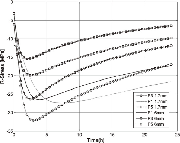
Calculated radial stresses in points p1, p3 & p5 for 6 mm and 1.7 mm thicknesses.

Fig. 15.

Calculated radial stresses in points p2, p4 & p6 for 6 mm and 1.7 mm thicknesses.

Fig. 16.

Calculated axial stresses in points p1, p3 & p5 for 6 mm and 1.7 mm thicknesses.

Fig. 17.

Calculated circumferential stresses in points p1, p3 & p5 for 6 mm and 1.7 mm thicknesses.

Fig. 18.

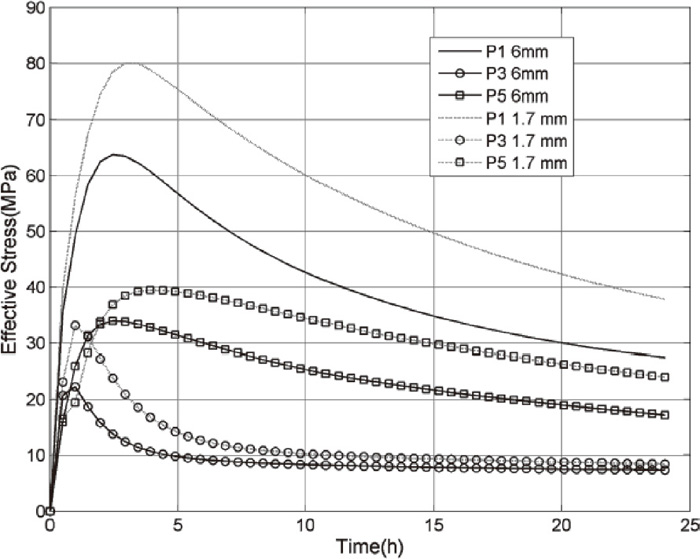
Calculated effective stresses in points p1, p3 & p5 for 6 mm and 1.7 mm thicknesses.

Figures 15, 16, 17, 18, 19 shows that the thinner strip coil exhibits higher stress levels and generally, peak stresses are reached around 2–3 hours.

Fig. 19.

Parameter influence on effective stress.

To investigate the coil parameters significance on the effective stress state and the average cooling rate a multiple linear regression analysis was performed. Input parameters were radius, height, thickness, coiler tension, strip crown ratio and crown shape. All parameters were fully factorial designed in two or three levels see Table 2. The calculated maximum von Mises effective stress obtained anywhere in the discretized domain was the response parameter. Interception terms up to a quadratic level were allowed and the initial temperature was set to 600°C in all simulations. Altogether 324 simulations were performed.

Table 2. Input parameters.

Parameter	Nr levels	Min. level	Med. level	Max. level
Radius [m]	3	0.85	0.95	1.05
Height [m]	3	0.8	1.0	1.2
Thickness [m]	3	0.001	0.005	0.01
Coiler tension [MPa]	3	25	50	75
α, Strip Crown factor	2	0.015		0.03
n, Crown shape	2	4		6

The regression analysis resulted in a coefficient of determination, R² = 0.982 and a RMS-error= 4.59 MPa. Figure 19 shows the influence of individual parameters on the effective stress while the others were kept at medium level values. The result shows that the thickness together with the coiler tension are the most significant parameters and that the strip shape profile parameters have no greater significant effect on the obtained maximum effective stress level.

The same linear regression model approach and input data as described above was further used to analyse the first two hours average cooling rate calculated as the difference between the initial and the domain mean temperature. Results are plotted in Fig. 20. An increased radius and height naturally resulted in a decreased cooling rate, the opposite holds for the thickness. It can be noted that the coiler settings do not have a significant influence on the average cooling rate. This analysis resulted in a coefficient of determination, R² = 0.998 and a RMS-error of 2.39•10⁻² °C/min.

Fig. 20.

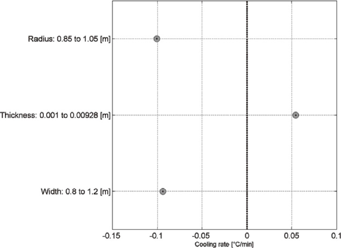
Parameter influence on average cooling rate.

4. Conclusions

The developed model shows a good agreement with measured temperature histories. The anisotropic thermal properties are important to incorporate in the model but the thermo-mechanically coupled effects are of secondary importance for the temperature predictions. In the previous model⁵⁾ a constant radial pressure to calculate gap zone properties was used, with good predictability but process variations in pressure due to strip shape, coiler settings and quality etc. was not able to be captured. An approximation that made the model static in both radial and axial directions and too generalized for real processes and further predictions of e.g. mechanical properties. Coiler settings and strip shape parameters under normal variation do have a low impact on the average cooling rate with exception for the coil tension that greatly influences the stresses. The coil dimensions and strip thickness has a major influence on the thermal gradients and thermally generated stresses. The number of interfacial zones has a key influence on the thermal conductivity, temperature gradients and consequently the stress states. The structural solution was not validated within this work but agrees well with previous works e.g. Park et al.⁶⁾ Furthermore was a linear elastic constitutive model implemented with assumption of no yielding, an assumption that holds when stresses are analysed from a macroscopic level i.e. when no nominal stress distribution across the thickness is considered.

The thermo-mechanical model approach though opens up for interesting possibilities of analyzing stress states evolved during the cooling procedure. Since the temperatures are relatively high in combination with slow cooling rates material will in some extent possibly undergo stress recovery in some parts across the domain which likely causes un-flatness effects like length-bow and cross-bow shaped material which in turn complicates downstream processes. This model approach solves the 24 hour transient thermo-mechanical coil cooling problem in a couple of seconds still with potential of even faster execution while optimized. Thus this approach is suitable for usage in optimizing or on-line applications.

Acknowledgements

The author wish to thank involved persons, Leif Bader, Erik Nymann and Magnus Gladh at SSAB EMEA works in Borlänge for experimental and technical support. Technical discussions with Prof. Lars-Erik Lindgren are gratefully appreciated.

References

• 1)   Y. J.  Jung,  G. T.  Lee and  C. G.  Kang: J. Mater. Process. Technol., 130–131 (2002), 195.
• 2)   R. B.  Sims and  J. A.  Place: Br. J. Appl. Phys., 4 (1953), 213.
• 3)   S.  Yanagi,  S.  Hattori and  Y.  Maeda: Proc. 7th Int. Conf. on Steel Rolling, ISIJ, Tokyo, (1998), 50.
• 4)   L.  Zheng-dong,  D. Q.  Jin,  I. V.  Samarasekera and  J. K.  Brimacombe: J. Iron Steel Res. Int., 12 (2005), 37.
• 5)   M.  Karlberg: ISIJ Int., 51 (2011), 416.
• 6)   S. J.  Park,  B-H.  Hong,  S. C.  Baik and  K. H.  Oh: ISIJ Int., 38 (1998), 1262.
• 7)   A.  Saboonchi and  S.  Hassanpour: J. Mater. Process. Technol., 182 (2007), 101.
• 8)   Y.  Xianglong,  J.  Zhengyi and  Y.  Quan: Adv. Mater. Res., 145 (2011), 111.
• 9)   A.  Saboonchi,  S.  Hassanpour and  A.  Hajiannezhad: J. Therm. Stress., 33 (2010), 521.
• 10)   M.  Karlberg: Iron Steel Rev., 59 (2015), 123.
• 11)   H.  Cho,  Y.  Cho,  Y.  Im,  J. K.  Lee,  J.  Kwak and  H.  Han: J. Mater.Process. Technol., 210 (2010), 907.
• 12)   B. B.  Mikic: Int. J. Heat Mass Tran., 17 (1974), 205.
• 13)   M. R.  Shridar and  M. M.  Yovanovich: J. Heat Transf., 118 (1996), 831.
• 14)   W. H.  Press,  S. A.  Teukolsky,  W. T.  Vetterling and  B. P.  Flannery: Numerical Recipes, the Art of Scientific Computing, Cambridge University Press, USA, (2007), 473.
• 15)   A-J. N.  Khalifa: Energ. Convers. Manage., 42 (2001), 491.
• 16)  Berechnungsblätter für den Wärmeübergang, Verein Deutscher Ingenieure-Wärmeatlas, 2nd ed., VDI-Verlag GmbH, Düsseldorf, (1974).
• 17)   A. D.  Kraus and  A.  Bejan: Heat Transfer Handbook, John Wiley & Sons Inc., New Jersey, (2003), 340.
• 18)   H.  Lundh: Grundläggande hållfasthetslära, Norstedts förlag, Stockholm, (1996).
• 19)   R. W.  Lewis,  K.  Morgan,  H. R.  Thomas and  K. N.  Seetharamu: The Finite Element Method in Heat Transfer Analysis, John Wiley & Sons Ltd., (1996), 99.