A Numerical Study about the Influence of a Bubble Wake Flow on the Removal of Inclusions

Abstract

The inclusion removal mechanism due to a bubble wake flow was studied using a water model and a three dimensional numerical model. In the experiments, a high-speed camera was used to record the bubble movement and the inclusion behavior connected to the flow. In the numerical model, the bubble induced fluid dynamics in the liquid was simulated using the volume of fluid (VOF) method. Also, the individual particle motion was tracked by the discrete phase model (DPM). A two-way coupling approach was used to model the interaction between the continuous phase and the discrete particles. The calculated results were compared with the experimental observations in the air-water-particle system. Calculations were also extended to an argon-steel-inclusion steelmaking system. The predictions show that the removal percent per bubble is increased with an increased bubble size. However, the inclusion removal percent per unit bubble volume can be improved by decreasing the bubble size. Also, the inclusion rising zone was found to be 1.625 and 5 times of the bubble size in width and height, respectively. It is also shown that the bigger inclusions are more easily removed compared to the smaller ones.

1. Introduction

The removal of inclusions in the steelmaking processes is of a high importance due to the ever-increasing stringent demands on improved steel properties. To achieve the aim of a lower inclusion concentration, researchers try to reveal the mechanism of the inclusion behavior in the metallurgical reactor systems. The inclusion removal mechanisms have been roughly categorized into three cases, namely, (1) the wall adhesion, 2) the inclusion buoyancy, 3) the bubble flotation.^1,2) The focus of this work is on the inclusion removal by bubble flotation. Specifically, the bubble is often generated by an inert gas stirring in the steel refining process. This injection accelerates the homogenization of the temperature and the chemical composition.

Computational Fluid Dynamics (CFD) simulations are widely used to study metal flows, especially where the experimental measurements are difficult or impossible to carry out due to the extreme critical operating environment. There are several phases, namely molten steel, gas, slag and inclusions, in a typical steelmaking vessel. These need to be considered in the simulation by using multiphase flow models.

“Clean steel” is of large interest to steel makers. Many researchers have studied the steelmaking flows by using different mathematical models and by focusing on different aspects, as shown in Table 1.^{1,3,4,5,6,7,8)} Here, the inclusions are part of a dynamics process which both includes the growth and removal of inclusions.^2,8,9) Meanwhile, the injected bubbles are also experiencing complicated phenomena such as a coalescence and breakup as well as a shape change.^3,10) It is hard to consider all the details in a quantitative model, especial for a large industrial scale reactor. In other words, more assumptions and empirical formula are needed to enable implementations to simulate a large scale reactor. Possible modelling attempts have been developed based on the different length scales (micro, meso, and macro). The focus has been on the single particle motion at the steel-slag interface in a micro way, the macroscopic transport of the inclusion concentration or the trajectories of the inclusion(s) in an industrial vessel, and the prediction of the inclusion deposition using meso-scale models.^{8,11,12,13,14)} A good review of this topic has recently been presented by Chao.¹⁵⁾

Table 1. Summary of mathematical models of multiphase flow in steelmaking.

Author	Year	Model	Turbulence	Reactor	Inclusion	Slag	Code
Sheng et al.1)	2002	E-E model (gas+liquid) PBM	k-ε model	ladle	Yes	No	Phoenics
Zhang et al.3)	2006	3D DPM (bubble)	k-ε model	CC Mold	Yes	No	Fluent
Li et al.4)	2008	3D VOF (interface, bubble)	k-ε model	ladle	No	Yes	Fluent
Schalk et al.5)	2009	3D VOF (interface)-DPM(bubble)	k-ε model	ladle	No	No	Fluent
Carlos et al.6)	2010	3D VOF (interface, bubble)	k-ε model	ladle	No	Yes	Fluent
Liu et al.7)	2011	3D VOF (interface)-DPM(bubble)	k-ε model	ladle	No	Yes	Fluent
Lou et al.8)	2013	3D CFD-PBM	k-ε model	ladle	Yes	No	Fluent
Present study	2016	3D VOF (bubble)-DPM (inclusion)	Laminar	Meso steel-bath	Yes	No	Fluent

The removal of inclusions by gas injection may be the result of bubble adhesion or bubble wake capture.^16,17) The attachment of particles on the rising bubbles has been the focus in most investigations. However, few numerical studies have been done to study the influence of the bubble wake flow on the removal of inclusions during steelmaking.¹⁷⁾ In this study, a gas bubbling water model has been built and it has been used to study the interaction between a bubble and a particle. Then a coupled VOF and DPM models was applied to investigate the single bubble-liquid-particle system. The simulations were validated against the water modeling results. Finally, the validated mathematical model was applied to investigate the influence of bubble wake flow on the removal of inclusions in the argon-steel-inclusion system.

2. Experiment

A schematic diagram of the experimental apparatus is shown in Fig. 1. This is a similar setup as was used in a previous study.¹⁸⁾ The rectangular vessel is made of plexiglass with an inner side length of 0.15 m. During the experiment, water was filled in the vessel to a height of 0.12 m. Thereafter, the gas (air) was supplied through a 60 mm long nozzle. The particles (D101 macroporous resin) were added to the liquid directly. Due to the similar densities of the water and the particles (1000 kg·m⁻³ vs 1060 kg·m⁻³), the particles were suspended in the water for a while. During the experiments, a high speed camera (MotionBLITZ Cube4) with a sample frequency of 1010 frames per second was used to record the bubble movement through the particle suspension. A strong illumination was used because the camera is very light sensitive.

Fig. 1.

Schematic diagram of the experimental apparatus. (1) square column; (2) gas nozzle; (3) regulating valve; (4) rotameter; (5) high speed camera; (6) personal computer; (7) illumination. (Online version in color.)

3. Mathematical Models

Simulations were carried out on the platform of ANSYS Fluent 14.5 by using a coupled VOF and DPM model. Specifically, the gas bubble was captured by the VOF model, while the particles (inclusions) were tracked by the DPM model.

3.1. VOF Model

The hydrodynamics of a continuous medium can be expressed by the continuity and momentum equations. For an incompressible Newtonian fluid, the equations are written as follows:

Continuity equation   

$$\nabla \cdot \left(\rho \mathbf{u}\right)=0$$(1)

Momentum equation   

$$\begin{array}{l}\frac{\partial }{\partial t}\left(\rho \mathbf{u}\right)+\nabla \cdot \left(\rho \mathbf{u}\mathbf{u}\right)=-\nabla p+\nabla \cdot \left[\mu \left(\nabla \mathbf{u}+\nabla {\mathbf{u}}^T\right)\right]\\ \hspace{1em}\hspace{1em}\hspace{1em}\hspace{1em}\hspace{1em}\hspace{1em}\hspace{1em}\hspace{1em}\hspace{0.5em}+\rho \mathbf{g}+{\mathbf{F}}_{\mathit{s}}+{\mathbf{F}}_{\mathit{d}}\end{array}$$(2)

where u is the velocity vector, ρ and μ are the fluid density and viscosity, respectively. Furthermore, p and g are the pressure and gravitational acceleration, respectively. The parameter F_s represents the surface tension force. The parameter F_d is momentum transfer term exerted by the discrete particles.

The VOF model is based on the solution of one set of momentum equations for the mixture of the phases, and one equation for the volume fraction of a fluid. The conservation equations are solved under the assumption of a laminar flow. The method of tracing an interphase boundary was achieved by solving the volume fraction continuity equation of one phase. Here, all phases are treated as incompressible with constant physical properties. Also, the temperature is constant in the bath and no chemical reactions are taken into account. A more detailed description can be found in the literature.¹⁰⁾

3.2. DPM Model

The particles are tracked by the discrete phase model (DPM). The trajectory of an individual particle is calculated by integrating the forces on the particle within a Lagrangian reference frame. This force balance equates the particle inertia with the forces acting on the particle, and can be shown as follows:   

$$\frac{d{\mathbf{u}}_p}{dt}={\text{F}}_D\left(\mathbf{u}-{\mathbf{u}}_p\right)+\frac{\mathbf{g}\left({\rho }_p-\rho \right)}{{\rho }_p}$$(3)

where u is the liquid velocity in the column, u_p is the velocity of the particle, ρ is the density of the liquid, ρ_p is the density of the particle. Furthermore, the term F_D (u−u_p) is the drag force per unit particle mass which can be expressed as follows:   

$${\text{F}}_D=\frac{18\mu }{{\rho }_p{d}_p^2}\frac{C_{D}Re}{24}$$(4)

where d_p is the particle diameter, the parameter Re is the relative Reynolds number, which is defined as follows:   

$$Re=\frac{\rho d_p\left|\mathbf{u}-{\mathbf{u}}_p\right|}{\mu }$$(5)

The drag coefficient C_D is calculated by:   

$$C_D=a_1+\frac{a_2}{Re}+\frac{a_3}{R{e}^2}$$(6)

where a₁, a₂ and a₃ are constant parameters depending on the Re value which are proposed by Morsi and Alexander.¹⁹⁾ It is noted that the DPM model is acceptable with the limitation that the discrete phase volume fraction is less than 12%.²⁰⁾ In this study, the particle volume fraction lies well below the constraint.

The effect of the discrete phase on the continuous phase is included by using a two-way coupling approach. This is accomplished by adding a momentum transfer source F_d in the continuous phase momentum equation. The term F_d exerted by the discrete particles is computed as:   

$${\mathbf{F}}_{\mathit{d}}=\left({\text{F}}_D\left(\mathbf{u}-{\mathbf{u}}_p\right)+\frac{{\mathbf{g}}_z\left({\rho }_p-\rho \right)}{{\rho }_p}\right){\dot{m}}_p\mathrm{\Delta }t$$(7)

where ${\dot{m}}_p$ is the mass flow rate of the particles and Δt is the particle time step.

3.3. Boundary Conditions and Solution Methods

The computational domain was a 40×40×120 mm³ square column. The geometric model was partitioned into uniform hexahedral cells. It was reported that the mesh independence could be reached with a mesh size of 0.5 mm for the current system.^21,22) By this way, the whole computational domain contained 1536 000 cells. No-slip boundary conditions were used at the walls. Also, a pressure outlet condition was employed at the outflow. In addition, the pressure-based method was used to separate and solve the model equations; the pressure–velocity coupling was solved by using the pressure-implicit with splitting of operators (PISO) method.²³⁾ In addition, a geometric reconstruction scheme was applied to track the free surface shape between the gas and the liquid. The convergence criteria were set to 1×10⁻³ for the residuals of all dependent variables. In order to maintain a stable solution, the time step should be restricted. A constant time step of 1×10⁻⁴ s was used in the present simulations, which corresponds to a maximum Courant number of 1. The calculations were carried out on a Win7 PC equipped with a 3.20 GHz Intel Core(TM) i7-3930K CPU. The computational time was about 6 days for one case.

4. Results and Discussion

4.1. Simulation Validation for an Air-water-particle System

The validation was carried out by comparing simulation and experimental results. The fluid properties used in the simulation and in the experiment are the same as shown in Table 2.

Table 2. Parameters used in the experiment and simulation.

ρp (kg/m3)	dp (mm)	ρl (kg/m3)	μl (kg/(m·s))	ρg (kg/m3)	μg (kg/(m·s))	σ (N/m)	db (mm)
1060	0.5	998.2	0.001	1.225	1.7894×10−5	0.0728	5.2

In the experiment, the gas flow rate was within the bubbling regime. Moreover, the individual bubble was supposed to be isolated with its own induced flow field. Particles have been added into the water and most of them are suspended in the liquid. A 5.2 mm bubble was formed at the bottom of the column. After the release of the bubble, it started to rise upward. Due to the bubble wake flow, some of the particles within a certain distance to the bubble were moving with the bubble. At one moment, a particle was found at the left side of the rising bubble (see Fig. 2(a)). The following process was tracked and is shown in Figs. 2(b)−2(f). Note, in order to make a good visualization, the other particles in the background and foreground were erased. At the same time, a simulation of the bubble rising process under the same condition was carried out. When the bubble reached the same position as it was in the experiment, a particle was added to the bubble’s left side. A similar scene was simulated in the mathematical model. The simulation results are shown in Figs. 2(g)−2(l).

Fig. 2.

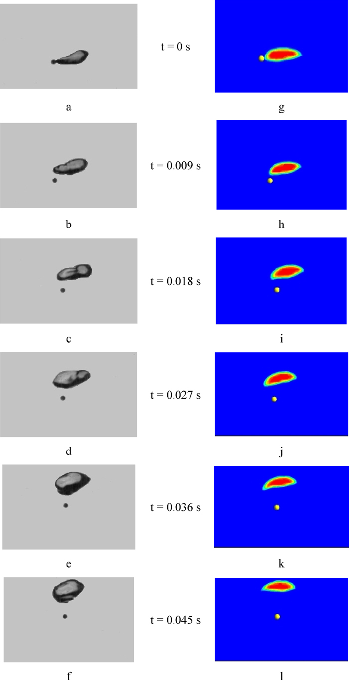
The experimental (a–f) and simulation (g–l) results of the particle’s movement caused by a bubble wake flow. (Online version in color.)

Comparisons between the experiment and the simulation results are given in Fig. 2. Both of the two methods reveal the fact that the particle is moving due to the bubble wake flow. Specifically, the movement of the bubble and the particle can be measured and calculated from the results. By measuring the movement of the bubble and the particle in 0.045 s, the average velocities of them are calculated. The measurements were done on three cases of a particle movement caused by a bubble wake. The average results are given in Table 3. The difference of the bubble velocities between simulations and the experiments is 2.5%. However, the particle velocities show a 28.9% deviation between predicted and measured results. The simulation of the bubble movement shows a good agreement with the experimental results. However, the particle modelling is less excellent. Still, the predictions give a satisfactory guidance on how to study the influence of a bubble wake flow on the particle removal behavior during injection of gas in a ladle.

Table 3. The movements and average velocities of the bubble and the particle within 0.045 s.

	DB (mm)	Dp (mm)	uB (m/s)	up (m/s)
Experiment	8.84	3.42	0.197	0.076
Simulation	9.1	2.45	0.202	0.054

Some important factors should be noted. In the experiment, a lot of particles were added in the water bath, but only one particle’s path was followed in the analysis. Also, the process took place in a three-dimensional space. However, the pictures taken from the high-speed camera were displayed in a two-dimensional way, the particle position in third dimension cannot be determined accurately. In the simulation, the particle location in the third dimension was assumed to be on the central axis of the bubble. Also, the parameters of the particle represented the average values of the macroporous resin particles used in the experiment. In addition, the bubble wake may be different due to the change of the bubble shape. With this in mind the results were deemed to be good and the model could be extended to the steelmaking system.

4.2. Bubble Wake Behavior in an Argon-steel-inclusion System

The coupled VOF and DPM model has been validated with water model experiments by focusing on a single bubble and a single particle. In that way, the mathematical model was applied to a steelmaking system which includes the argon bubble, the molten steel and the inclusions. The properties of these fluids are shown in Table 4.

Table 4. Parameters used in the simulation of the steelmaking system.

ρp (kg/m3)	ρg (kg/m3)	ρl (kg/m3)	μg (kg/(m·s))	μl (kg/(m·s))	σ (N/m)
3000	1.6228	7100	2.125×10−5	0.006	1.8

Several assumptions have been made to study the bubble wake flow in the argon-steel-inclusion system numerically. The inclusions (with a total number of N_p) are supposed to only be initially in the lower part of the computational domain. In addition, it is assumed that there is no interaction between inclusions. Also, a single spherical bubble is located below the inclusion region (see Fig. 3(a)). From Figs. 3(b) to 3(d), the bubble rises up in the bath due to the buoyancy force. During the bubble’s movement, it will experience a passage through the inclusion zone. Due to the effect of the bubble wake flow, some of the particles can rise below the bubble. Also, the distribution of the particles in Fig. 3(d) shows that the bubble rises in a zigzag way, which is in accordance with the results from a previous study.¹⁰⁾

Fig. 3.

The passing of a bubble through the inclusion zone where d_B=10 mm, d_p=100 μm, N_p=10000. (Online version in color.)

The area of the bubble wake flow which can make the inclusions rise is defined as the inclusion rising zone.¹⁶⁾ To study the width of the rising zone, the particles’ velocity field of Fig. 3(b) is shown in Fig. 4. The velocities are almost symmetrical in this case, because the bubble rises linearly during this short period. The width of the inclusion rising zone is supposed to be within the two black lines in Fig. 4. The two black lines are drawn based on the inclusions’ movement. Specifically, the inclusions which show notable movement are distinguished to the rest of the inclusions. The distance between the two lines is 26 mm, which is 1.625 times that of the bubble width (16 mm). In Fig. 3(d), a few particles follow behind the bubble, so the top limitation of the rising zone is supposed to be terminated at this bubble location. The height of the rising zone is 80 mm, which gives a value of 5 with respect to the height. In the study of Yang et al.,¹⁶⁾ the basic scope of the rising zone was found to be 1.5 times that of the bubble size in width and 5.5 times in height. Thus, the simulation values show good agreement with the literature results.

Fig. 4.

The particles’ velocity of Fig. 3(b). (Online version in color.)

The velocity field and pressure field distribution of Fig. 3(c) on a central vertical cross section are shown in Fig. 5. As shown in Fig. 5, the particle entrainment due to the bubble induced flow field is demonstrated. It is seen that the flow field is asymmetric and that the vortex appears separately. Therefore, the distribution of the moving inclusions is also asymmetric. It can be found that the vortex on the right hand side of the bubble is full of particles. This is due to the low pressure region presented in the vortex (see Fig. 5(b)).

Fig. 5.

The velocity field and pressure field of Fig. 3(c). (Online version in color.)

4.3. Effect of Bubble Diameter in the Argon-steel-inclusion System

To quantify the inclusion removal percent due to the bubble wake, the inclusions which are present above the horizontal interface of the suspension are defined as the removed inclusions N_p-r. These inclusions are supposed to be removed due to a bubble wake flow. Obviously, the removal percent per bubble R can be calculated by dividing the total particle number with the number of the removed inclusions. Furthermore, the removal percent per unit bubble R_unit can be calculated by dividing the bubble volume ratio with the removal percent per bubble.   

$$R=\frac{N_{p-r}}{N_p}$$(8)

  

$$R_{unit}=\frac{N_{p-r}}{N_p}/\frac{V}{V_{unit}}$$(9)

where V is the bubble volume and V_unit is the reference bubble volume.

Three different bubble diameters were studied, namely, 5 mm, 10 mm and 16 mm with 100 μm inclusions. The effect of the bubble diameter on the removal percent is shown in Fig. 6. It is seen that the removal percent per bubble is increased with an increased bubble size (see Fig. 6(a)). It is quite understandable that the bubble induced wake flow is stronger as the bubble size becomes larger. Therefore, more inclusions can be moved by the flow if the bubbles are large compared to if they are small. However, the inclusion removal percent of per unit bubble volume is the opposite. As is shown in Fig. 6(b), the highest inclusion removal percent of unit bubble volume is produced by the smallest bubble (here, the volume of the 5 mm bubble is considered as the reference bubble volume). In another way, if a big bubble is separated into several small bubbles, the inclusion removal percent is improved. The results suggest that small bubble is preferred in real industrial operations. Possible methods to obtain small bubbles include a change of the type, size or the wettability of the bottom tuyere.^8,18)

Fig. 6.

The effect of the bubble diameter on (a) the inclusion removal percent per bubble and (b) the inclusion removal percent per unit bubble volume. (Online version in color.)

4.4 Effect of Inclusion Diameter in the Argon-steel-inclusion System

Three types of inclusion diameter were studied, namely, 1 μm, 10 μm and 100 μm with a 10 mm bubble. The effect of the inclusion size on the removal percent is shown in Fig. 7. It can be seen that the inclusion removal percent is higher with a larger inclusion size. The smaller inclusions are more difficult to remove. It was shown that the number of inclusions affected by the bubble was higher for smaller inclusions.¹⁶⁾ That is to say the small inclusions are more easily controlled by the flow field, but it does not mean the inclusions are removed. The effective inclusion removal requires that the particles surpass certain height without turning back. There are several vortices in the bubble wake flow field (see Fig. 5(a)); it is also a dynamic process which may include wake shedding. The larger the inclusions the stronger the buoyancy force, this helps the inclusions to pass the flow eddy. Therefore, the smaller inclusions experience a higher probability to move backwards. This is one fact that explains why smaller inclusions are difficult to be removed in the industrial operation.

Fig. 7.

The effect of the inclusion size on the inclusion removal percent. (Online version in color.)

4.5. Discussion

All the simulation results are based on several assumptions as mentioned in Section 4.2. The real situation is much more complex than the current system. The purpose of the paper is to study the single bubble wake flow on the inclusion removal behavior. This represents only one of the metal flow phenomena in a real steelmaking process. The results supply basic rules of this behavior under a simplified situation which may not be possible in reality. However, this fundamental work is a necessary supplement for the deep understanding of the bubble wake flow in metallurgical operations.

5. Conclusions

A coupled VOF and DPM model was used to study the influence of a bubble wake flow on the particle removal behavior. The model was validated by a water model experiment by comparing the movement of a single particle due to a single bubble. The average bubble velocity and particle velocity from simulation are of 2.5% and 28.9% differences compared to the experimental results. The qualitative agreement shows that the numerical methods can be used for this kind of system. Thereafter, the mathematical model was used to study the phenomenon in the argon-steel-inclusion system. The results show that the inclusion rising zone is 1.625 times of the bubble size in width and 5 times of the bubble size in height. It is also shown that the inclusion removal percent per bubble is increased from 2.3% to 18.9% by increasing the bubble diameter from 5 mm to 16 mm. However, the highest inclusion removal percent per unit bubble volume is produced by the smallest bubble; it is 2.9 times larger for the 5 mm bubble compared to the 16 mm bubble. In addition, the simulation results show that smaller inclusions (6.8% to 1 μm inclusions) are harder to remove than the larger inclusions (8.1% to 100 μm inclusions).

Acknowledgments

Yonggui Xu would like to extend his sincere appreciation to the CSC (China Scholarship Council) for financial support of his PhD studies at KTH-Royal Institute of Technology, Sweden.

Nomenclature

α_g: Value of gas volume fraction [-]

μ: Viscosity [kg·m⁻¹·s⁻¹]

ρ: Density [kg·m⁻³]

σ: Surface tension coefficient [N·m⁻¹]

p: Pressure [Pa]

g: Gravitational acceleration [m·s⁻²]

t: Time [s]

u: Velocity [m·s⁻¹]

F_s: Surface tension force [N·m⁻³]

C_D: drag coefficient [-]

F_d: Drag force [N·m⁻³]

d_p: Inclusion diameter [m]

D_B: Movement of bubble [m]

D_p: Movement of particle [m]

N_p: Total number of inclusions [-]

N_p-r: Number of removal inclusions [-]

R: Inclusion removal percent per bubble [-]

R_unit: Inclusion removal percent per unit bubble [-]

Re: Reynolds number [-]

References

• 1)   D. Y.  Sheng,  M.  Söder,  P.  Jönsson and  L.  Jonsson: Scand. J. Metall., 31 (2002), 134.
• 2)   M.  Söder,  P.  Jönsson and  L.  Jonsson: Steel Res. Int., 75 (2004), 128.
• 3)   L.  Zhang,  J.  Aoki and  B. G.  Thomas: Metall. Mater. Trans. B, 37 (2006), 361.
• 4)   B.  Li,  H.  Yin,  C. Q.  Zhou and  F.  Tsukihashi: ISIJ Int., 48 (2008), 1704.
• 5)   S. W.  Cloete,  J. J.  Eksteen and  S. M.  Bradshaw: Prog. Comput. Fluid Dyn., 9 (2009), 345.
• 6)   C. A.  Llanos,  S.  Garcia-Hernandez,  J. A.  Ramos Banderas,  J. d. J.  Barreto and  G.  Solorio-Diaz: ISIJ Int., 50 (2010), 396.
• 7)   H. P.  Liu,  Z. Y.  Qi and  M. G.  Xu: Steel Res. Int., 82 (2011), 440.
• 8)   W.  Lou and  M.  Zhu: Metall. Mater. Trans. B, 44 (2013), 762.
• 9)   T.  Emi: Lectures in Tundish Technology, Royal Institute of Technology, Stockholm, (1997).
• 10)   Y.  Xu,  M.  Ersson and  P.  Jönsson: Steel Res. Int., 86 (2015), 1289.
• 11)   J.  Strandh,  K.  Nakajima,  R.  Eriksson and  P.  Jönsson: ISIJ Int., 45 (2005), 1597.
• 12)   Y.  Yang,  P. G.  Jönsson,  M.  Ersson and  K.  Nakajima: Steel Res. Int., (2014), 341.
• 13)   P.  Ni,  L. T. I.  Jonsson,  M.  Ersson and  P. G.  Jönsson: Int. J. Multiph. Flow, 62 (2014), 152.
• 14)   P.  Ni,  L.  Jonsson,  M.  Ersson and  P.  Jönsson: Metall. Mater. Trans. B, 45 (2014), 2414.
• 15)   C.  Chen: Ph. D. Thesis, Royal Institute of Technology, Stockholm, (2015).
• 16)   H. L.  Yang,  P.  He and  Y. C.  Zhai: ISIJ Int., 54 (2014), 578.
• 17)   Y.  Kang,  L.  Yu and  D.  Sichen: Ironmaking Steelmaking, 34 (2007), 253.
• 18)   Y.  Xu,  M.  Ersson and  P.  Jönsson: Metall. Mater. Trans. B, 46 (2015), 2628.
• 19)   S.  Morsi and  A.  Alexander: J. Fluid Mech., 55 (1972), 193.
• 20)  Ansys 14.5 manual, ANSYS, Inc., USA, (2012).
• 21)   Y.  Zhang,  M.  Liu,  Y.  Xu and  C.  Tang: Chem. Eng. Sci., 73 (2012), 55.
• 22)   Y.  Xu,  M.  Liu and  C.  Tang: Chem. Eng. J., 222 (2013), 292.
• 23)   R. I.  Issa,  B.  Ahmadi-Befrui,  K. R.  Beshay and  A. D.  Gosman: J. Comput. Phys, 93 (1991), 388.