On-line Energy Allocation Based on Approximate Dynamic Programming for Iron and Steel Industry

Abstract

Energy allocation in iron and steel industry is the assignment of available energy to various production users. With the increasing price of energy, a perfect allocation plan should ensure that nothing gets wasted and no shortage. This is challenging because the energy demand is dynamic due to the changes of orders, production environment, technological level, etc. This paper try to realize on-line energy resources allocation under the situation of dynamic production plan and environment based on typical energy consumption process of steel enterprises. Without definite analytical model, it is a tough task to make the energy allocation plan tracks the dynamic change of production environment in real time. This paper proposes to deal with dynamic energy allocation problem by interactive learning with time-varying environment using Approximate Dynamic Programming method. The problem is formulated as a dynamic model with variable right-hand items, which is an updated energy demand obtained by on-line learning. Reinforcement learning method is designed to learn the energy consumption principle from the historical data to predict energy consumption level corresponding to current production environment and the production plan in future horizon. Using the prediction results, on-line energy allocation plan is made and its performance is demonstrated by comparison with static allocation method.

1. Introduction

Energy is the foundation of modern industry and is facing huge and tremendous demand increase by the driving of the sustained economic growth, which results in rapid demand increase of primary and secondary energy. As one of the typical energy-intensive industry, the energy consumption level of an iron & steel enterprise accounts for about 15% of the countrywide quantity of China. Traditional research on iron and steel planning and optimization usually focuses on production itself.¹⁾ However, with the increase of energy price, the cost of energy consumption covers 20–35% of the whole iron & steel production cost. And, the comprehensive energy consumption of China is much higher than that of the world with the energy utilization being only 30%. As a common indicator to measure the energy consumption level of iron & steel industry, the comprehensive energy consumption per ton steel of China is much higher than that of developed countries such as United States, Japan, South Korea, etc. Therefore, there is considerable optimization potential.

Iron & steel production is a complicated system with multi-process, multi-equipment and multi-energy. The production and energy consumption interrelates and interact with each other in iron & steel industry that the consumption of more than 20 kinds of energy media including electricity, gas, steam, water, oxygen, etc. are consumed, converted and regenerated simultaneously. During this course, the energy demand of each process, the energy supply capacity, the holding capacity, the safety, the emission restriction and the dynamism of all aforementioned need be taken into account. Unthoughtful allocation and use of energy will undoubtedly leads to the more cost of products, more pollution, more emission, and so on. Therefore, it has been a major task for energy management department to insure continuous, safe, and economical energy supply, and efficient energy utilization. The development of energy-saving strategy has become an increasingly prominent task, which can be accomplished by implementing technological progress and equipment renovation, or by improving management level. The implementation of the former two strategies usually involves huge cost due to equipment and production technology replacement, while the last strategy aims at reducing energy consumption level by exploring advanced management tools, which from the view of cost, are feasible ways to improve the utilization rate of energy in iron & steel industry.

Currently, the common challenge that most iron & steel enterprise confronts is no deterministic model or rule about energy consumption and the deficiency of energy allocation from the view of the whole factory. The current situation of traditional energy management can be summarized as follows. First, energy is allocated based on the production plan at the beginning of the production horizon and remains unchanged till the end of the horizon. Second, allocation of energy usually focuses on a single type, for example, gas system, electricity system, etc. In real-world industry, any change such as machine breakdown, the arrival of rush order and temporary change of orders, the instability of workers operating level, the change of equipment operating status will make the energy production environment deviate from original status, which will affect the energy demand. And, coupling among different types of energy exists along with the production all the time, for example, during the course of consuming primary energy (electricity, coal, nature gas, etc.) in ironmaking, steelmaking and rolling process, secondary energy (coke oven gas, blast furnace gas, Lindz.Donawitz gas, steam and so on) are generated, and extra gas and steam can be used to generate electricity.

The key task of energy allocation is to comprehensively consider the consumption and regeneration in the whole production horizon. The goal of energy allocation is to reduce the total production cost while guarantee the smooth production. Traditional research on energy allocation method, static or dynamic, usually assume known and fixed parameters in the horizon, however, dynamic energy demand in almost all practical situation requires the allocation plan of energy closely track the change of production plan so as to increase the utilization rate. Without considering the above mentioned energy features during the course of energy allocation will inevitably lead to energy wastage and emission. Therefore, traditional fixed-demand based method no longer meets the practical requirements, and the research on new on-line allocation of energy is needed.

The idea of using real-time information to make decision can be found in the research of inventory management, that is, design efficient method to obtain accurate demand estimation in future lead time when signing order contract.^2,3,4,5) In production area, some rescheduling methods have been reported to deal with unexpected real-time events.⁶⁾ However, the research with real-time information updates has not been found, and most reports on energy allocation in production focus on deterministic case. Boukas and Haurie⁷⁾ studied electric arc furnace scheduling problem with energy constraints consideration. The objective is to determine the start time for processes in each production cycle subject to energy control constraints, priority constraints and availability constraints of shared equipments. Hierarchical method is used for solving. Javier⁸⁾ researched the jobshop facility integrated manufacturing and control system under electricity real-time-pricing in his dissertation. The effect of energy and waste on production scheduling is taken into account to minimize the total production cost including energy cost. Ruiz et al.⁹⁾ studied real-time on-line optimization of the utilities system of a production site, the optimization objective is the overall system cost minimization under the constraints of equipment, fuels and electricity pricing, emissions limits, quotas and rights. Applications using real-world data in refineries and chemical plants demonstrated the optimization results. Cai et al.¹⁰⁾ developed a large-scale dynamic optimization model for a long-term energy systems planning. The model describes the energy management system as networks of a series of energy flows, transferring in/out energy resources to end users over a number of periods. The system is helpful for tackling dynamic and interactive characteristics of the energy management system in examining impacts of energy and environmental policies, regional development strategies and emission reduction measures.

The on-line energy allocation problem in this paper originates from the actual need of typical energy-intensive process in iron & steel plant. This research tries to allocate energy among all users in real time, considering the consumption of primary energy, the regeneration and conversion of secondary energy, and the dynamic features of production environment. The dynamism caused by the above-mentioned changes and the coupling or uncertainty among these factors will affect the energy demand and consumption level, only the latest information-based energy allocation plan could meet the requirement the practical production. This is also the motivation and focus of this paper.

Some operations in iron and steel production will last a few hours, wherein production status changes frequently. Thus the on-line energy allocation belongs to multi-stage sequential decision problem. Dynamic Programming (DP) based solving method is usually used to deal with multi-stage optimization problems. DP has wide application in the area of engineering, operations research, economics.^11,12,13,14) However, DP records all suboptimal decision for all possible state from a certain time point to the end of the horizon, the burden of computation and storage increases exponentially with the state space dimension.¹⁵⁾ This kind of “curse of dimensionality” limits DP from large scale application.¹⁶⁾ In recent years, to overcome “curse of dimensionality”, Approximate Dynamic Programming (ADP) has gradually attracted researchers attention with the basic idea of replacing exact computation of all states at each stage with estimated cost function.¹⁷⁾ Generally, ADP uses Cost-to-go function approximation¹⁸⁾ to construct parameters from sample data in discrete state space, and gradually improves its performance through on-line interaction with environment. In ADP, critic module approximates cost-to-go function, and the action module generates action. The critic module evaluates the performance of action, based on which the action module carries out adjustment. Therefore, ADP method will not be affected by inaccurate parameters and is appropriate for solving problems with unknown models. Schmid¹⁹⁾ designed an ADP-based optimization method for ambulances real-time scheduling problem, which is featured as: an appropriate vehicle needs to be dispatched and sent to the required sits immediately once a request emerges, and after having completed a request the vehicle should be relocated to its next waiting location. The test on real-world data of a city shows that compared with traditional assignment rules ADP improved the average response time by 2.89%. Ganesan et al.²⁰⁾ addressed the taxi-out time prediction problem in airport and developed ADP-based solving method. The experimental results of 5 US airports shows 14–50% improvement compared with regression models. Simao et al.²¹⁾ used the largest truckload motor carrier in the United States as the background and studied the large-scale fleet scheduling problem, considering multiple dynamic characteristics (driver type, location, domicile, and work time constraints, etc.). The authors combined ADP with mathematical programming, which provided satisfying solutions with good performance in the costs of hours-of-service, cross-border driver management, hiring drivers, etc.

To sum up, ADP exhibits advantages in solving real-time or dynamic problems, implying that it is suitable for the on-line energy allocation problem studied in this paper. Most research on energy allocation is based on given demand (which is usually obtained by estimation or simple computation, for example, weighted average) and lack of real-time interaction with environment. In real world, in the process of production plan execution, production situation is difficult to remain the same as the beginning when time moves forward, naturally the energy demand will change accordingly and the initial allocation plan is no longer accurate. This paper proposes a demand updates based on-line energy allocation method, which is a rolling prediction method taking full advantage of ADP’s superiority in dealing with time-varying problems. On-line energy allocation model with variable right hand items is established, ADP is used to estimate the energy demand based on the latest production information, then the updated demand prediction results are used to generate energy allocation among all users.

2. Problem Description and Modeling of On-line Energy Allocation

In iron & steel industry, there are usually 6 energy-intensive processes - Coking, Sintering, Ironmaking, Steelmaking, Hot rolling and Cold rolling, as shown in Fig. 1. Different processes need different types of energy to ensure the production. Some types of energy, like electricity and gas, are required by almost all processes, others like oxygen, are required by ironmaking, steelmaking. Energy allocation problem can be described as follows: Dynamically allocate each kind of energy media among users in given horizon so as to minimize the total energy consumption, considering primary energy, secondary energy and energy conversion simultaneously.

Fig. 1.

Illustration of energy consumption and regeneration in all processes of iron & steel enterprise.

The task of energy prediction is to provide the energy management department with accurate amount of energy needed in certain time periods in future. To make the energy allocation plan closely follow up with any change of production environment, this paper proposes an on-line energy allocation method as follows: the planning horizon is divided into limited time periods. The real-world energy consumption data, the production plan and the environment information change with time periods, based on which energy demand prediction in each period is implemented and embedded in the on-line energy allocation plan. In general, the on-line energy allocation problem is learning and dynamic programming-based optimization. The overall structure of the proposed framework is based on dynamic programming, at each stage of which a linear programming model is formulated to express the allocation subproblem, and the real-time energy demand is obtained by the embedded ADP prediction module. In nature, this framework is environment interaction-based allocation method. The basic idea of energy allocation at each stage is shown by Fig. 2.

Fig. 2.

The basic idea of energy allocation at each stage of on-line energy allocation.

As the core part of the proposed framework, energy demand prediction estimates the quantity of energy needed to complete the future production based on history energy consumption data and real-time information. The accuracy of prediction is affected by many factors. First, production data that approaches the prediction time period expresses current production status more accurately than those faraway ones, therefore, using “near” data may bring relative accurate prediction results. Second, the prediction accuracy is affected by the design of input & output variables and the method of modeling. To determine the input & output variables, the factors that affect energy consumption level should be figured out through analysis or experiments. Based on analysis and practical experience, the quantity of energy used has close relationship with production conditions among which production yield and air temperature have significant impact. The role of energy is to serve and guarantee the production, then it is easy to understand that the consumption level of all kinds of energy is directly proportional of the quantity of yield. More production means more consumption of gas, electricity, water and so on. In addition, iron & steel production is temperature-related and sometimes the hating process starts from air temperature, therefore the difference of air temperature has significant impact on the demand of gas or electricity. Consequently, in the prediction model, planned yield and air temperature are designed as the input variables, and the items (include demand and regeneration) to be predicted as the output variables.

The on-line energy demand prediction in this paper is carried out by ADP, which interacts with environment in a dynamic manner to realize estimation. The implementation of ADP composes of two stages, learning and testing. At the stage of learning, the ADP learning procedures are designed to learn the consumption principle from the sample data, which are updated in a rolling way with time so as to approach the prediction environment as close as possible. At the stage of testing, the energy demand is estimated based on the learnt results, the production plan and other environmental information.

2.1. Mathematical Model for Energy Allocation

The parameters of on-line energy allocation problem are listed as follows:

t: Time period index, t = 1,2,…, T, T is the planning horizon

i: Process index, i = 1,2,…, I, I is the number of processes

j: Energy media index, j = 1,2,…, J, J is the number of energy media

x_ijt: Allocated quantity of energy j in time period t at process i

c_jt: Unit cost of energy j in time period t

S_jt: Supply quantity of energy j in time period t

α_ij: Secondary energy productive rate of generating energy j at process i

$p_{ijt}^s$: Unit penalty for shortage of energy j in time period t at process i

$p_{ijt}^e$: Unit penalty for excess of energy j in time period t at process i

d_ijt: Demand of energy j in time period t at process i

The purpose of on-line energy allocation is to achieve optimal allocation and improve energy efficiency. The objective is set as: minimization of energy consumption cost, energy shortage penalty and energy waste penalty.   

$$\begin{array}{l}minz=\sum _{t=1}^T\sum _{i=1}^I\sum _{j=1}^J{c}_{jt}{x}_{ijt}+\sum _{t=1}^T\sum _{i=1}^I\sum _{j=1}^J{p}_{ijt}^{s}max\left\{0,d_{ijt}-x_{ijt}\right\}\\ \hspace{1em}\hspace{1em}\hspace{1em}+\sum _{t=1}^T\sum _{i=1}^I\sum _{j=1}^J{p}_{ijt}^{e}max\left\{0,x_{ijt}-d_{ijt}\right\}\end{array}$$(1)

The constraints considered are energy supply constraints (2) and variable values constraints (3). Constraints (2) require that in any time period, for any kind of energy media, the consumption quantity cannot be more than the available quantity, where the available quantity comprises of the supply capacity in current time period and the secondary energy generated in immediately previous time period.   

$$\sum _{i=1}^I{x}_{ijt}\le S_{jt}+\sum _{i=1}^I{\alpha }_{ij}{x}_{ij,t-1},\mathrm{\hspace{0.17em} }\forall j,\mathrm{\hspace{0.17em} }{x}_{ijt}|{}_{t=0}=0$$(2)

  

$$x_{ijt}\ge 0,\forall i,\forall j,\forall t$$(3)

The energy allocation problem expressed by (1), (2) and (3) involves time-based multi-stage decision and can be solved by Dynamic Programming using the following state transition equations:   

$$\begin{array}{l}{f}_t\left(S_t\right)=\underset{x_{ijt}\in X_{ijt}}{min}\left[c_t\left(S_t,x_{ijt}\right)+f_{t-1}\left(S_{t-1}\right)\right]\\ f_0\left(S_0\right)=0\end{array}$$(4)

  

$$\begin{array}{l}{c}_t\left(S_t,x_{ijt}\right)=\sum _{i=1}^I\sum _{j=1}^J{c}_{jt}{x}_{ijt}+\sum _{i=1}^I\sum _{j=1}^J{p}_{ijt}^{s}max\left\{0,d_{ijt}-x_{ijt}\right\}\\ \hspace{1em}\hspace{1em}\hspace{1em}\hspace{1em}\hspace{0.5em}+\sum _{i=1}^I\sum _{j=1}^J{p}_{ijt}^{e}max\left\{0,x_{ijt}-d_{ijt}\right\}\end{array}$$(5)

Where, c_t(S_t,x_ijt) is the stage value of energy consumption cost, energy shortage penalty and energy waste penalty. Traditionally, the above state transition equations of DP are based on static parameters, meaning that the parameters in (4) and (5) remain unchanged from the beginning to the end of the time horizon. To deal with real-world dynamic energy allocation problem with time varying parameters, ADP-based solving method is proposed and elaborated in subsection 2.2 and section 3.

2.2. Mathematical Model for Energy Demand Prediction

The problem presented in subsection 2.1 comprises multi-stage decisions, each of which is based on the real-time energy demand prediction. To obtain the value of d_ijt in each period t, ADP algorithm is designed to realize on-line energy prediction. ADP algorithm is characterized as self-learning and self-adaptive, making it suitable for time-varying complex system and dynamic complicated task, especially for the problems without analytical model. Based on such features, ADP fits well for the addressed on-line energy allocation problem. The details are as follows.

Parameters:

α₀ Initial value of learning parameter

K_α A big number that denotes the decay rate of learning parameter

P₀ Initial value of exploration probability

K_P A big number that denotes the decay rate of exploration probability

ε_E Threshold value of exploration stopping criterion

ε_L Threshold value of learning stopping criterion

γ Discount factor

k Prediction horizon

To solve a problem, ADP usually first analyze and find state variables that could well express problem features, then design value function, action and contribution for each state. Based on the analysis of input & output variables, the system state of process i in time period t is set as: ${\overrightarrow{s}}_{it}=\left\{s_{1it},s_{2t}\right\}$ for energy demand prediction, where ${\overrightarrow{s}}_{it}$ is the system state space of process i in time period t, s_1it is the yield of process i in time period t and s_2t is the air temperature in time period t. The action is denoted by a_it, which corresponds to the predicted value of d_ijt in time period t at process i. The system state transition function is defined as:   

$${\overrightarrow{s}}_{i,t+1}=S^M\left({\overrightarrow{s}}_{it},d_{ijt},W_{i,t+1}\right)$$

Where W_i,t+1 denotes all the information that arrives between period t and t+1. Since accuracy is the most important performance index for energy demand prediction problem, the contribution function d_t$\left({\overrightarrow{s}}_{it},d_{ijt}\right)$ is defined as: the absolute value of the difference between the actual value $d_{ijt}^{ACT}$ and predicted value $d_{ijt}^{PRE}$ with respect to the demand of process i, energy j in time period t, that is,   

$$d_t\left({\overrightarrow{s}}_{it},d_{ijt}\right)=\left|d_{ijt}^{ACT}-d_{ijt}^{PRE}\right|$$(6)

With the discount factor γ(0 < γ < 1), the objective is to minimize the expectation of the sum of discount prediction deviation.   

$$\underset{d_{ijt}\in D_{ijt}}{min}E\left\{\sum _{t=0}^{\infty }\gamma d_t\left({\overrightarrow{s}}_{it},d_{ijt}\right)\right\}$$(7)

Where D_ijt is the action space. P$\left(s^{\prime }|{\overrightarrow{s}}_{it},d_{ijt}\right)$ is the state transition probability at state s′. To solve (5), Bellman equation is adopted to establish the following model:   

$$\begin{array}{l}{V}_t\left({\overrightarrow{s}}_{it}\right)=\underset{d_{ijt}\in D_{ijt}}{min}\left[d_t\left({\overrightarrow{s}}_{it},d_{ijt}\right)+\gamma E\left\{V_{t+1}\left({\overrightarrow{s}}_{i,t+1}\right)|{\overrightarrow{s}}_{it},d_{ijt}\right\}\right]\\ \hspace{1em}\hspace{1em}\hspace{1em}=\underset{d_{ijt}\in D_{ijt}}{min}\left[d_t\left({\overrightarrow{s}}_{it},d_{ijt}\right)+\gamma \left(\sum _{s^{\prime }\in S}P\left(s^{\prime }|{\overrightarrow{s}}_{it},d_{ijt}\right)V_{t+1}\left({\overrightarrow{s}}_{i,t+1}\right)\right)\right]\end{array}$$(8)

For most problems, it is difficult to obtain the knowledge of state transition probability P$\left(s^{\prime }|{\overrightarrow{s}}_{it},d_{ijt}\right)$, thus Robbins-Monro stochastic approximation method based ADP algorithm is used to realize the prediction of (8), that is, to obtain the value of d_ijt for each type of energy media in each process. To simplify the derivation procedures of solvable expression of V_t(${\overrightarrow{s}}_{it}$) for each process i in time period t, we use s_t as the simplified expression of s_it and use a_t to simplify a_it (the action to determine the predicted value of d_ijt, the amount of energy j to be used at process i in time period t) from Eqs. (9), (10), (11), (12), (13), (14).   

$$\begin{array}{l}{V}_t\left(s_t\right)=\underset{a_t\in A_t}{min}\left(d_t\left(s_t,a_t\right)+\gamma E\left\{V_{t+1}\left(s_{t+1}\right)|s_t\right\}\right)\\ \hspace{1em}\hspace{1em}\hspace{0.5em}=\underset{a_t\in A_t}{min}\left(d_t\left(s_t,a_t\right)+\gamma \sum _{s^{\prime }\in S}P\left(s^{\prime }|s_t,a_t\right)V_{t+1}\left(s^{\prime }\right)\right)\end{array}$$(9)

At each decision point, it is difficult to solve exactly the value function at state s_t because of computational burden. Iterative estimation is used to approximate the value function. Let ${\overline{V}}_t$(s_t) be the approximation of value function obtained by iterative estimation, ${\overline{V}}_t^0$ be the initial approximate value, and ${\overline{V}}_t^{n-1}$ be the approximate value after n−1 iterations. At the beginning of iteration, the value of action a₀ is obtained by solving the following equation,   

$$\begin{array}{l}{a}_0=\underset{a\in A_0}{argmin}\left(d_0\left(s_0,a\right)+\gamma E\left\{{\overline{V}}_1\left(s_1\right)|s_0\right\}\right)\\ \hspace{1em}=\underset{a\in A_0}{argmin}\left(d_0\left(s_0,a\right)+\gamma \sum _{s^{\prime }\in S}{P}_0\left(s^{\prime }|s_0,a\right){\overline{V}}_1\left(s^{\prime }\right)\right)\end{array}$$(10)

By state transition function s_t+1=S^M (s_t,a_t,W_t+1), the next state s₁ is get based on the initial state s₀, then iterative decision is carried out. According to Bellman equation with discount factor, the optimal value function $V_t^{*}$(s_t) at state s_t can be calculated by,   

$$V_t^{*}\left(s_t\right)=\underset{a\in A_t}{min}\left(d_t\left(s_t,a\right)+\gamma \left(\sum _{s^{\prime }\in S}P\left(s^{\prime }|s_t,a\right)V_{t+1}^{*}\left(s^{\prime }\right)\right)\right)$$(11)

According to Bellman theory, for each state-decision tuple (s, a), the optimal value function is obtained by solving the following equation:   

$$\begin{array}{l}{V}^{*}\left(s,a\right)=\sum _{s^{\prime }\in S}P\left(s^{\prime }|s,a\right)d\left(s,a\right)\\ \hspace{1em}\hspace{1em}\hspace{1em}\hspace{0.5em}+\gamma \left[\sum _{s^{″}\in S}P\left(s^{″}|s,a\right)\underset{a^{\prime }\in A}{min}{V}^{*}\left(s^{″},a^{\prime }\right)\right],\forall s,\forall a\end{array}$$(12)

Here, s′ and s″ are the possible states obtained by implementing action a at state s. $P\left(s^{\prime }|s,a\right)$ and $P\left(s^{″}|s,a\right)$ the corresponding state transition probabilities. a″ is the action that minimize the value function at state s″. Considering the difficulty of obtaining the knowledge of state transition probability, the learning version of (12) is expressed as:   

$$\begin{array}{l}{V}_t^n\left(s,a\right)=\left(1-{\alpha }_{n-1}\right)V_t^{n-1}\left(s,a\right)\\ \hspace{1em}\hspace{1em}\hspace{1em}\mathrm{\hspace{0.17em} }\hspace{0.5em}+{\alpha }_{n-1}\left[d_t\left(s,a\right)+\gamma \underset{a^{\prime }\in A}{min}{V}_{t+1}^{n-1}\left(s^{″},a^{\prime }\right)\right],s,s^{″}\in S\text{, }a\in A\end{array}$$(13)

Where α (0<α<1) is the learning parameter, which is updated by:²²⁾   

$${\alpha }_{n-1}=\frac{{\alpha }_0}{1+u},\mathrm{\hspace{0.17em} }u=\frac{{\left(n-1\right)}^2}{K+n-1}$$(14)

K is a big number, α₀ = 0.7.¹³⁾

Finally, based on learning version of value function approximation in (13) and the design of state variables for energy prediction problem, the learning version of value function for state-action 2-tuple $\left({\overrightarrow{s}}_{it},d_{ijt}\right)$ is as follows:   

$$\begin{array}{l}{V}_t^n\left({\overrightarrow{s}}_{it},d_{ijt}\right)=\left(1-{\alpha }_{n-1}\right)V_t^{n-1}\left({\overrightarrow{s}}_{it},d_{ijt}\right)\\ \hspace{1em}\hspace{1em}\hspace{1em}\hspace{1em}\hspace{1em}\hspace{0.5em}+{\alpha }_{n-1}\left[d_t\left({\overrightarrow{s}}_{it},d_{ijt}\right)+\gamma \underset{a^{\prime }\in D_{ijt}}{min}{V}_{t+1}^{n-1}\left({\overrightarrow{s}}_{i,t+1},a^{\prime }\right)\right]\end{array}$$(15)

Where, ${\overrightarrow{s}}_{it},{\overrightarrow{s}}_{i,t+1}\in S,\mathrm{\hspace{0.17em} }{d}_{ijt}\in D_{ijt}$. The learning parameter α decays according to (14).

The ADP-based learning procedures can be illustrated by Fig. 3.

Fig. 3.

The flow chart of ADP-based learning procedures.

3. Design of Prediction Algorithm Based on ADP

In this section, the detailed procedures of ADP-based energy allocation algorithm will be presented. To obtain real-time energy demand, first, the system state, action, contribution function and other parameters of energy prediction are designed. After a specific initialization, the learning and testing stages of the proposed algorithm are elaborated. The purpose of initialization is to assign initial values to the actions with respect to value functions of all initial states. At the stage of learning, sample data is fed to ADP one by one and iteratively until the improvement of value function stops. At the stage of testing, new input of the state to be predicted will be given to the ADP to get energy demand, based on which the energy allocation in corresponding time period is carried out. The detailed steps of on-line energy allocation are as follows.

Step 1 Determine state, action and contribution function of energy prediction problem. Set prediction horizon and the length of the time window.

Step 2 Determine and discretize the state space and the action space, the value functions V$\left({\overrightarrow{s}}_{it},d_{ijt}\right)$ corresponding to all state-action pair $\left({\overrightarrow{s}}_{it},d_{ijt}\right)$ are initialized to 0.

Step 3 Let n = 1, exploration stage begins, get the exploration probability P, if P ≤ ε_E then go to Step 4; otherwise generate a random number m from a uniform distribution, then choose any action $d_{ijt}\in D_{ijt}$ when m < P (P is the exploration probability), or choose greedy action $d_{ijt}\in D_{ijt}$ (the action corresponding to minimal V value). When a state ${\overrightarrow{s}}_{it}$ is visited for the first time, choose action $d_{ijt}\in D_{ijt}$ randomly since V$\left({\overrightarrow{s}}_{it},d_{ijt}\right)$ is initialized to 0. The value of exploration probability P is updated by,   

$$P_{n-1}=\frac{P_0}{1+u_P},\mathrm{\hspace{0.17em} }{u}_P=\frac{{\left(n-1\right)}^2}{K_P+n-1}$$

Calculate contribution c_t$\left({\overrightarrow{s}}_{it},d_{ijt}\right)$, get next state ${\overrightarrow{s}}_{i,t+1}$, update V$\left({\overrightarrow{s}}_{it},d_{ijt}\right)$ according to (14), n=n+1, go to Step 5.

Step 4 Start learning, let n=1, choose action d_ijt from D_ijt using greedy criterion, calculate contribution c_t$\left({\overrightarrow{s}}_{it},d_{ijt}\right)$, get next state ${\overrightarrow{s}}_{i,t+1}$, update V$\left({\overrightarrow{s}}_{it},d_{ijt}\right)$ by (13), n=n+1, go to next step.

Step 5 Continue learning with training matrix, Learning ends when V$\left({\overrightarrow{s}}_{it},d_{ijt}\right)$ converges $\left(\left|V^n-V^{n-1}\right|\le {\epsilon }_L\right)$ for each 2-tuple $\left({\overrightarrow{s}}_{it},d_{ijt}\right)$, then go to next step.

Step 6 After learning, the obtained V$\left({\overrightarrow{s}}_{it},d_{ijt}\right)$ table includes optimal action for each state, then each unknown variable d_ijt is solved by looking up the V$\left({\overrightarrow{s}}_{it},d_{ijt}\right)$ table based on the corresponding system state ${\overrightarrow{s}}_{it}$.

The overall scheme of dynamic demand update-based ADP algorithm for on-line energy allocation can be summarized as: Dynamic programming (DP) method is adopted at the outermost layer of the scheme so that the planning horizon is divided into multiple stages, each of which corresponds to a subproblem that is formulated as a linear programming (LP) model based on the prediction result of ADP. The subproblem can be optimally solved by CPLEX. ADP is used at each stage to accomplish exact estimation of demand through iterative learning because it is difficult to obtain accurate energy demand with respect to the updated production environment without necessary knowledge of energy consumption principle.

4. Experimental Results Based on Real-world Data

In order to demonstrate the performance of the proposed ADP algorithm for on-line energy allocation problem, the real-world energy data in a Chinese iron & steel enterprise is used. Six production processes including sintering, coking, ironmaking, steelmaking, hot rolling and cold rolling are considered. The proposed algorithms have been implemented using Language C++ on a PC with Intel (R) Core (TM) 2 Duo CPU (2.33 GHz) and Windows XP operating system. The distribution of energy consumption and regeneration among production processes considered in this paper is shown by Table 1, in which the abbreviations are: BFG - Blast Furnace Gas, COG - Coke Oven Gas, LDG - Lindz.Donawitz Gas, LO₂- Low-pressure oxygen, HO₂ - High-pressure oxygen, Ar – Argon, MSteam - Medium-pressure steam, LSteam - Low-pressure steam.

Table 1. Distribution of energy consumption and regeneration among all considered production processes.

Process	BFG	COG	LDG	LO2	HO2	N2	Ar	MSteam	LSteam	Electricity
Sintering		√						+	√	√
Coking	√	√ +				√		√	√ +	√
Ironmaking	√ +	√		√	√	√			√	√ +
Steelmaking			√ +		√	√	√		√ +	√
Hot rolling	√	√	√						+	√
Cold rolling		√		√		√			√	√

‘√’ means consumption of the energy in the corresponding process, ‘+’ means regeneration of the energy in the process

4.1. Performance of ADP for Prediction

As the core part of on-line energy allocation approach, the accuracy of energy demand prediction will directly affect the final performance. The real-world energy data of steelmaking process (shown in Table 2) is used to show the prediction results.

Table 2. Real-world data of energy consumption in steelmaking process.

t	S1it	S2t	LDG	HO2	N2	Ar	LSteam	Electricity
	(ton)	(°C)	(m3)	(m3)	(m3)	(m3)	(kg)	(kwh)
1	25.21	1.5	10.4	59.4	33.7	1.50	25.2	68.8
2	23.46	2.3	10.9	60.7	36.1	1.60	23.9	64.6
3	26.60	11.6	10.5	59.5	31.8	1.40	28.5	61.9
4	24.37	15.6	10.5	59.0	33.9	1.40	30.2	64.4
5	22.34	22.2	11.3	59.5	27.6	1.40	30.6	70.2
6	23.88	23.5	10.1	59.8	27.9	1.30	32.5	68.0
7	24.65	29.0	9.7	60.1	31.3	1.50	27.9	73.5
8	24.36	27.0	9.8	59.6	31.5	1.50	29.5	68.9
9	22.18	24.4	10.2	60.4	34.1	1.60	32.0	79.7
10	17.42	19.0	14.3	63.3	38.1	1.70	45.5	90.4
11	18.13	10.5	14.7	60.6	46.6	1.90	50.6	103.1
12	17.41	5.8	16.0	62.8	45.2	1.70	43.2	108.4
13	18.08	2.2	15.0	60.0	45.4	1.70	36.0	107.0
14	20.90	7.3	12.1	60.0	40.4	1.60	44.0	82.8
15	23.42	9.8	9.8	60.3	38.9	1.56	37.0	76.5
16	14.67	16.6	11.4	60.5	35.1	2.00	9.0	90.9
17	21.67	21.9	12.2	60.5	34.8	1.73	16.0	81.6
18	25.95	26.6	9.9	58.7	34.0	1.62	9.0	73.6
19	29.72	28.0	10.0	58.6	33.8	1.84	7.0	73.4
20	30.56	27.2	9.9	58.4	33.4	1.64	8.0	72.0
21	29.24	23.4	9.4	59.1	33.5	1.60	12.0	74.0
22	29.78	20.1	10.5	58.0	34.7	1.56	14.0	73.0
23	24.16	8.6	12.5	58.9	36.0	1.65	15.0	78.8
24	32.30	4.5	10.5	59.8	38.8	1.60	11.3	74.0
25	33.16	3.6	9.0	57.0	37.0	1.60	11.0	74.5
26	28.52	6.0	10.2	56.56	39.79	1.57	7.4	73.2
27	30.94	8.6	10.9	56.3	39.9	1.49	7.0	76.3
28	26.90	12.8	12.1	51.9	39.6	1.50	7.0	82.9
29	33.34	21.1	10.0	55.9	34.8	1.57	9.0	72.1
30	28.90	24.8	9.8	58.3	32.5	1.63	9.5	69.6
31	32.74	28.3	10.0	56.1	34.0	1.57	9.2	71.4
32	32.10	29.7	9.6	54.9	32.3	1.63	9.4	69.8
33	32.19	24.2	9.9	55.6	32.7	1.55	9.3	68.9

In theory, d_ijt has infinite number of possible values in the action space, which is unmanageable for the real-world problem addressed, therefore this paper discretizes the action space into finite number of values. Other algorithm parameters are listed in Table 3. As the core part of the proposed method, the accuracy of energy demand prediction will directly affect the whole performance, therefore the results of ADP for on-line and static energy demand prediction are summarized in Table 4. Here the length of prediction horizon is set as 5 time periods, the on-line prediction is implemented by up-to-date data of each time period while the static prediction is based on the data prior to the prediction horizon. It can be seen from the data in Table 3 that the on-line prediction deviations keep in relative lower level than the static method with average values being 3.7512% and 4.1768% respectively. Occasionally, the prediction deviation is larger than 5%, on one hand, this is due to the possibility that more impact factors should be extracted from the practical production and designed as the components of state vector. On the other hand, as a kind of data-based algorithm, the performance of ADP is affected by the size and quality of sample data.

Table 3. Parameter values for ADP algorithm.

Parameter	α0	Kα	P0	KP	εE	εL	γ	k
Value	0.7	8×1013	1	500	0.00001	0.05	0.9	5

Table 4. On-line and static prediction results for steelmaking process.

4.2. Experimental Results of on-line Energy Allocation Based on ADP

The data used for energy allocation experiment comprise of three parts: real-world data, data calculated from real data and random data generated based on the consumption rule. The planning horizon T=15 (hours), the number of processes I=6, the number of energy media J=10. The penalty $p_{ijt}^s$ and $p_{ijt}^e$ are generated based on the overall consideration of unit energy cost c_jt and the priority of meeting demand. Using these data, the on-line energy allocations for 6 processes are carried out. The production plans of these processes along the planning horizon are given by Table 5, where the data has reasonable changes compared with stable real-world data in Table 2 in order to test the performance of the proposed method. In Table 5, the data under S_2t represent the air temperature and remain the same values for all the processes. To verify the performance of demand update-based dynamic programming method for energy allocation problem, static programming method is designed, which determines the energy allocation of each time period without considering the impact between adjacent processes. Here static means the energy demand is predicted at the beginning of planning and keeps unchanged along of the horizon, while the demand for on-line framework is updated in each time period.

Table 5. The production plans of all considered processes.

(unit: S1it – ton, S2t –°C)
Time period	Sintering		Coking		Ironmaking		Steel making		Hot rolling		Cold rolling
	S1it	S2t	S1it	S2t	S1it	S2t	S1it	S2t	S1it	S2t	S1it	S2t
1	41.53	15.6	7.09	15.6	23.20	15.6	20.64	15.6	26.73	15.6	9.70	15.6
2	48.68	22.2	6.18	22.2	26.17	22.2	25.16	22.2	27.55	22.2	5.17	22.2
3	41.37	23.5	7.61	23.5	16.07	23.5	31.25	23.5	15.70	23.5	7.23	23.5
4	29.30	29.0	8.75	29.0	18.06	29.0	28.19	29.0	28.31	29.0	6.77	29.0
5	28.03	27.0	9.61	27.0	15.43	27.0	19.24	27.0	19.31	27.0	7.72	27.0
6	37.34	24.4	12.51	24.4	19.99	24.4	30.45	24.4	30.32	24.4	8.01	24.4
7	39.65	19.0	9.38	19.0	20.19	19.0	19.54	19.0	31.21	19.0	8.89	19.0
8	40.51	10.5	9.91	10.5	23.87	10.5	16.35	10.5	30.64	10.5	7.98	10.5
9	41.83	5.8	12.46	5.8	25.51	5.8	23.58	5.8	13.54	5.8	6.90	5.8
10	42.33	2.2	10.93	2.2	19.78	2.2	21.13	2.2	16.26	2.2	6.93	2.2
11	36.61	7.3	10.00	7.3	23.58	7.3	21.86	7.3	20.44	7.3	5.27	7.3
12	54.63	9.8	11.86	9.8	16.42	9.8	33.46	9.8	28.38	9.8	7.93	9.8
13	28.33	16.6	8.80	16.6	15.77	16.6	30.84	16.6	17.87	16.6	9.32	16.6
14	28.27	21.9	13.24	21.9	28.40	21.9	14.43	21.9	15.19	21.9	8.19	21.9
15	37.95	26.6	8.09	26.6	17.79	26.6	26.39	26.6	31.45	26.6	6.25	26.6

Tables 6, 7, 8, 9, 10, 11 present the comparison results of energy allocation plans of all processes by the proposed demand update-based on-line method and static method. The differences (marked in bold) between on-line and static frameworks can be seen in these tables. Such differences are caused by the different method of energy demand prediction. Further, different quantity of energy allocated in the prior time period results in different quantity of regeneration which will affect the available amount of energy to be used in the subsequent time period. Recall that energy consumption cost, energy shortage penalty and energy waste penalty are considered in the objective function, then, with limited available quantity of energy, the goal of energy allocation is to seek a comprehensive plan with overall consideration and balance of these objectives. That’s why the quantity of energy allocated to each process is not simply determined by the production yield and in the obtained results the quantity of energy is not proportional to the production yield.

Table 6. Comparison between on-line and static energy allocation for sintering process.

Time period	On-line results			Static results
	COG (m3)	LSteam (kg)	Electricity (kwh)	COG (m3)	LSteam (kg)	Electricity (kwh)
1	4.00	14.20	35.70	4.00	14.20	35.70
2	3.90	14.80	51.50	3.90	14.80	51.50
3	3.88	14.80	37.00	3.88	14.80	37.00
4	3.72	10.60	42.00	3.72	10.60	42.00
5	3.72	10.60	42.00	3.72	10.60	42.00
6	3.74	13.20	38.80	3.74	13.20	38.80
7	3.80	12.20	38.25	3.80	12.20	38.25
8	3.75	8.20	44.00	3.75	8.20	44.00
9	3.69	9.55	41.50	3.69	9.55	41.50
10	3.69	9.55	41.50	3.69	9.55	41.50
11	3.71	10.70	43.50	3.71	10.70	43.50
12	3.96	10.75	53.50	3.96	10.75	53.50
13	3.72	10.60	42.00	3.72	10.60	42.00
14	3.72	10.60	42.00	3.72	10.60	42.00
15	3.74	13.20	38.80	3.74	9.40	38.80

Table 7. Comparison between on-line and static energy allocation for coking process.

Time period	On-line results						Static results
	BFG (m3)	COG (m3)	N2 (m3)	MS team (kg)	LS team (kg)	Elect ricity (kwh)	BFG (m3)	COG (m3)	N2 (m3)	MS team (kg)	LS team (kg)	Elect ricity (kwh)
1	509.61	88.37	17.59	13.15	3.15	26.50	510.11	87.87	17.59	13.15	3.15	26.50
2	702.29	130.19	12.71	15.70	2.35	29.50	496.70	112.38	12.71	15.03	2.35	29.50
3	743.00	193.50	11.02	15.82	4.91	29.50	542.08	193.50	11.02	16.30	4.91	29.50
4	590.50	138.50	6.52	16.60	3.46	28.50	590.50	138.50	6.52	13.93	3.46	28.50
5	585.00	123.50	4.37	16.00	3.62	28.50	585.00	123.50	4.37	14.41	3.62	28.50
6	474.00	200.50	6.49	15.62	2.80	26.00	570.50	122.50	2.64	14.32	3.59	27.00
7	624.50	135.00	4.25	15.06	2.62	28.50	624.50	82.56	4.25	10.72	2.62	28.50
8	623.67	126.00	5.00	14.54	3.74	27.50	407.25	143.00	5.89	10.62	4.72	27.00
9	603.19	144.00	2.04	13.86	4.90	22.50	566.39	156.50	2.84	13.40	6.01	22.00
10	651.00	114.50	3.14	14.04	5.25	25.00	681.00	144.50	3.82	14.60	6.38	23.00
11	617.00	98.50	3.39	15.12	3.38	28.00	513.00	93.50	2.59	13.70	3.93	29.50
12	616.50	151.00	3.19	14.90	3.18	26.00	581.67	156.50	2.84	13.07	6.01	22.00
13	662.00	140.50	6.59	15.00	2.33	29.00	412.39	140.50	6.59	13.09	2.33	29.00
14	474.00	200.50	6.49	15.62	2.80	26.00	570.50	122.50	2.64	11.95	3.59	27.00
15	482.50	163.00	3.30	16.42	4.10	29.00	482.50	163.00	3.30	15.80	4.10	29.00

Table 8. Comparison between on-line and static energy allocation for ironmaking process.

Time period	On-line results							Static results
	BFG (m3)	COG (m3)	LO2 (m3)	HO2 (m3)	N2 (m3)	LS team (kg)	Elect ricity (kwh)	BFG (m3)	COG (m3)	LO2 (m3)	HO2 (m3)	N2 (m3)	LS team (kg)	Elect ricity (kwh)
1	701.00	7.82	20.87	0.67	16.38	7.54	54.00	701.00	7.82	20.68	0.67	16.38	7.54	54.00
2	664.00	6.72	21.72	0.58	23.10	12.16	56.50	664.00	6.72	21.62	0.58	23.10	12.16	56.50
3	709.80	7.46	25.08	0.90	22.34	9.00	56.50	715.50	7.46	24.96	0.90	22.34	9.00	56.50
4	705.50	7.11	18.90	0.80	22.80	8.51	57.50	705.50	7.11	18.78	0.80	22.80	8.51	57.50
5	722.00	7.32	23.21	0.84	22.60	7.90	56.00	681.74	7.32	23.11	0.84	22.60	7.90	56.00
6	705.50	7.11	20.68	0.80	22.80	8.51	57.50	605.39	7.11	20.58	0.80	22.80	8.51	57.50
7	705.50	7.11	22.79	0.80	22.80	8.51	57.50	597.84	7.11	22.69	0.80	22.80	8.51	57.50
8	674.50	7.23	24.70	0.61	19.30	8.85	53.00	674.50	7.23	24.70	0.61	18.94	8.85	53.00
9	674.50	6.73	22.70	0.60	18.50	7.97	53.50	513.00	2.44	28.50	0.45	27.50	8.76	56.00
10	711.50	7.60	20.52	0.79	21.00	8.10	53.50	711.50	7.60	20.17	0.79	21.00	8.10	53.50
11	585.07	6.22	23.04	0.61	18.60	8.92	53.50	479.89	6.22	22.69	0.61	19.30	8.92	53.50
12	715.50	7.46	27.30	0.90	23.60	9.00	56.50	715.50	7.46	26.95	0.90	23.60	9.00	56.50
13	669.25	8.13	27.62	0.70	23.80	14.00	55.00	708.50	8.13	27.52	0.70	23.80	14.00	55.00
14	626.50	5.63	25.00	0.50	18.60	10.90	55.00	541.01	5.63	25.00	0.50	22.45	10.90	55.00
15	705.50	7.11	25.60	0.80	21.46	8.51	57.50	662.20	7.11	25.60	0.80	21.46	8.51	57.50

Table 9. Comparison between on-line and static energy allocation for steelmaking process.

Time period	On-line results						Static results
	LDG (m3)	HO2 (m3)	N2 (m3)	Ar (m3)	LSteam (kg)	Electricity (kwh)	LDG (m3)	HO2 (m3)	N2 (m3)	Ar (m3)	LSteam (kg)	Electricity (kwh)
1	11.10	60.00	35.00	1.40	33.92	78.00	11.10	60.00	35.00	1.40	33.92	78.00
2	10.00	52.74	31.50	1.46	27.82	69.50	10.00	52.74	31.50	1.46	27.82	69.50
3	9.90	52.00	37.00	1.55	59.00	77.00	9.90	58.50	34.00	1.55	20.00	73.00
4	9.80	58.00	33.50	1.59	21.38	74.50	9.80	59.00	33.00	1.59	20.78	73.50
5	11.60	51.11	33.00	1.45	32.72	78.00	11.60	51.11	33.00	1.45	32.72	78.00
6	9.90	53.87	34.00	1.66	20.40	74.00	9.90	53.87	34.00	1.65	20.00	73.00
7	12.50	57.69	28.37	1.56	36.94	85.00	12.50	57.69	28.98	1.56	36.94	85.00
8	14.30	52.07	42.00	1.36	38.86	100.00	14.30	52.07	42.00	1.36	38.86	100.00
9	11.10	60.00	37.00	1.58	31.02	74.50	10.50	58.50	34.50	1.66	21.20	74.00
10	12.10	58.05	39.50	1.62	33.18	82.00	12.10	58.05	39.50	1.62	33.18	82.00
11	11.10	60.00	37.00	1.40	31.02	74.50	11.10	60.00	37.00	1.40	31.02	74.50
12	10.00	56.50	38.00	1.59	19.54	74.50	10.10	56.93	33.50	1.61	21.90	71.00
13	10.00	54.15	36.00	1.60	20.20	75.50	10.10	54.15	33.50	1.60	21.90	71.00
14	14.30	61.50	42.00	1.33	38.86	100.00	14.30	61.50	20.35	1.33	38.86	100.00
15	9.90	58.50	34.00	1.60	19.00	73.50	9.90	59.22	34.00	1.60	19.00	71.50

Table 10. Comparison between on-line and static energy allocation for hot rolling process.

Time period	On-line results				Static results
	BFG (m3)	COG (m3)	LDG (m3)	Electricity (kwh)	BFG (m3)	COG (m3)	LDG (m3)	Electricity (kwh)
1	67.50	51.50	33.41	98.00	67.00	52.50	33.41	99.50
2	70.50	49.50	26.49	98.50	70.00	51.50	21.05	98.50
3	64.00	58.50	36.30	116.00	64.00	36.76	36.30	116.00
4	68.50	49.50	31.08	95.50	67.50	51.50	26.23	104.00
5	61.50	56.00	28.80	112.00	65.50	56.50	24.00	113.50
6	68.50	49.50	34.70	95.50	70.00	51.50	29.28	98.50
7	71.50	50.00	25.08	97.00	70.00	51.50	20.23	98.50
8	60.00	49.50	23.30	95.50	69.00	48.50	17.91	95.00
9	66.00	63.00	30.29	119.00	66.00	63.00	23.88	119.00
10	66.00	63.00	30.40	119.00	39.73	21.49	29.75	119.00
11	57.50	58.00	31.10	111.00	57.50	58.00	31.10	111.00
12	61.50	51.00	26.45	96.50	69.00	15.02	20.91	97.00
13	57.00	65.00	25.70	114.50	57.00	65.00	25.70	114.50
14	64.00	58.50	36.30	116.00	64.00	58.50	31.96	116.00
15	72.50	49.50	32.70	96.50	70.00	51.50	28.50	98.50

Table 11. Comparison between on-line and static energy allocation for cold rolling process.

Time period	On-line results					Static results
	COG (m3)	LO2 (m3)	N2 (m3)	LSteam (kg)	Electricity (kwh)	COG (m3)	LO2 (m3)	N2 (m3)	LSteam (kg)	Electricity (kwh)
1	49.50	0.10	29.80	149.69	224.12	49.50	0.10	29.80	147.23	227.03
2	49.00	0.10	20.23	129.17	244.78	49.00	0.12	23.23	158.00	247.64
3	48.00	0.10	18.13	155.00	269.67	43.93	0.12	18.63	158.00	261.03
4	49.00	0.10	26.15	158.00	237.54	28.69	0.10	26.15	158.00	234.88
5	49.50	0.10	23.51	138.78	267.59	49.00	0.10	23.51	132.05	263.46
6	50.00	0.10	31.13	138.88	250.63	50.00	0.10	30.52	133.61	247.97
7	51.50	0.30	14.03	203.76	226.97	15.78	0.35	14.03	191.38	221.81
8	54.50	0.10	27.91	245.50	175.39	51.00	0.35	28.38	234.50	165.32
9	51.00	0.35	18.84	196.91	234.60	51.00	0.35	18.84	189.30	235.56
10	50.47	0.30	25.62	203.92	260.00	34.71	0.35	25.62	196.59	257.50
11	38.15	0.25	25.21	215.16	203.87	51.00	0.35	28.38	203.47	218.29
12	51.00	0.10	24.16	180.50	234.76	29.65	0.10	29.42	169.00	238.12
13	49.00	0.10	32.41	129.26	270.50	49.00	0.10	31.32	124.21	269.50
14	49.00	0.02	17.18	153.15	239.56	23.95	0.02	17.18	146.20	238.45
15	51.00	0.10	23.52	151.62	244.40	50.50	0.19	23.52	152.22	242.90

To visualize the merit of on-line allocation framework, the accumulations of the objectives of on-line and static frameworks along the horizon are drew in Fig. 4. It can be observed from Fig. 4 that the two frameworks of the presented processes have almost equal cost at the first period, and the on-line framework exhibits obvious superiority than static framework in almost all the after periods. With respect to the cost accumulations along the horizon, the on-line allocation approach outperforms the static one in each process and the overall plant. The prediction accuracy of ADP has been proved by the experiments using real-world data in Table 4. Therefore, as time progress, the superiority of on-line framework will be increasingly obvious because on-line allocation framework is based on on-line prediction of energy demand and static framework is based on constant demand. We can conclude that by using ADP to interactively learn with time-varying environment and provide accurate energy demand, the energy allocation plan could track the dynamic change of production environment and complete the production task with lower energy cost. The proposed demand update-based dynamic programming method could realize the requirement of on-line energy allocation both in effectiveness and running time.

Fig. 4.

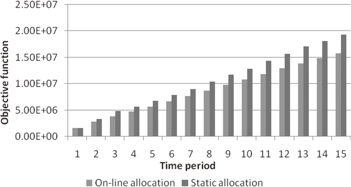
Objective comparison between on-line and static frameworks of all considered processes.

5. Conclusions

This paper studied the energy allocation problem with demand updates. An ADP-based solving method is proposed to deal with the random and time-varying features. The overall methodology is designed as a dynamic programming with each stage determining the optimal allocation plan based on updated energy demand. ADP algorithm is designed to accomplish real-time energy demand prediction, based on which the decision problem at each stage is formulated as a linear programming model that is optimally solved by CPLEX. Compared with static scheme, the proposed on-line energy allocation method shows obvious superiority in effectiveness and stability.

Acknowledgement

This research is partly supported by National Natural Science Foundation of China (Grant No. 71302161, 61374203), National 863 High-Tech Research and Development Program of China (Grant No. 2013AA040704), the Fund for Innovative Research Groups of the National Natural Science Foundation of China (No. 71321001), and State Key Laboratory of Synthetical Automation for Process Industries Fundamental Research Funds (Grant No. 2013ZCX02).

References

• 1)   L. X.  Tang,  G. S.  Wang and  Z.  Chen: Oper. Res., 62 (2014), 772.
• 2)   H. Y.  Huang,  S. P.  Sethi and  H. M.  Yan: IIE Trans., 37 (2005), 775.
• 3)   S. P.  Sethi,  H.  Yan and  H.  Zhang: J. Optim. Theory Appl., 108 (2001), 253.
• 4)   S. P.  Sethi,  H. M.  Yan and  H. Q.  Zhang: Oper. Res., 51 (2003), 321.
• 5)   Q.  Feng,  G.  Gallego,  S. P.  Sethi,  H. M.  Yan and  H. Q.  Zhang: J. Optim. Theory. Appl., 124 (2005), 137.
• 6)   L. X.  Tang,  Y.  Zhao and  J. Y.  Liu: IEEE Trans. Evol. Comput., 18 (2014), 209.
• 7)   E. K.  Boukas and  A.  Haurie: Ann. Oper. Res., 26 (1990), 289.
• 8)   A. M.  Javier: Oklahoma State University, Doctor Dissertation, (1999).
• 9)   D.  Ruiz and  C. A.  Ruiz: Comput.-Aid., Chem. Eng., 27 (2009), 1455.
• 10)   Y. P.  Cai,  G. H.  Huang,  Z. F.  Yang,  Q. G.  Lin,  B.  Bass and  Q.  Tan: Int. J. Energy Res., 32 (2008), 988.
• 11)   R.  Bellman and  S.  Dreyfus: Applied Dynamic Programming, Princeton University Press, Princeton, (1962), 1.
• 12)   T.  Borgers and  R.  Sarin: Econ. Theor., 77 (1997), 1.
• 13)   J.  Dalton and  S. N.  Balakrishnan: Math. Comput. Model., 23 (1996), 175.
• 14)   P.  Werbos: General System Yearbook, Vol. 22, Society for General Systems Research, Louisville, (1977), 25.
• 15)   W. B.  Powell: Approximate Dynamic Programming: Solving the Curses of Dimensionality, Wiley-Interscience, New York, (2007).
• 16)   D. E.  Kirk: Optimal Control Theory: An Introduction, Prentice-Hall, Englewood Cliffs, (1970), 1.
• 17)  Handbook of Learning and Approximate Dynamic Programming eds. by J. Si, A. G. Barto, W. B. Powell and D. Wunsch, IEEE Press and John Wiley & Sons, New York, (2004), 1.
• 18)   R. E.  Bellman: Dynamic Programming, Princeton University Press, Princeton, (1957).
• 19)   V.  Schmid: Eur. J. Oper. Res., 219 (2012), 611.
• 20)   G.  Rajesh,  B.  Poornima and  S.  Lance: Qual. Reliab. Eng. Int., 26 (2010), 717.
• 21)   H. P.  Simao,  J.  Day,  A. P.  George,  T.  Gifford,  J.  Nienow and  W. B.  Powell: 4th Int. Workshop on Freight Transportation and Logistics, INFORMS, Cesme, (2009), 178.
• 22)   A.  Gosavi: Simulation-based optimization: parametric optimization techniques and reinforcement learning, Kluwer Academic, Norwell, MA, (2003).