Reliability of Inclusion Statistics in Steel by Stereological Methods

Abstract

In this paper, we investigate the reliability of estimating of inclusion size distribution and number density in steel by using stereological methods. The magnitude of the inclusion concentration in steel is evaluated by the total oxygen and the assumed average inclusion sizes. The principles of Schwartz-Saltykov (SS) and modified SS (MSS) methods are introduced. A simulation model is developed to disperse particles with a predefined particle size distribution (PSD) randomly into a three dimensional (3D) space. A series of test planes are generate to measure the two dimensional (2D) PSD and particle number density (PND) on the cross-sections (CS). The SS and MSS methods are applied to investigate the reliability of the translation between the 3D and 2D information of the system, such as the 2D and 3D PSD and PND. The influence of predefined 3D PSD on the reliability of the stereological methods are studied, such as mono sized, lognormal and normal distributions. The effect of the representative group diameters in the discretized groups for SS and MSS methods is investigated as well.

1. Introduction

Nonmetallic inclusions in steel largely decrease the mechanical performance of the steel products,^1,2) such as strength, toughness, fatigue property, plasticity, surface smoothness and corrosion resistance. The requirements of the control of inclusions in steel products become more and more serious.³⁾ It is an everlasting topic to improve the cleanliness of the steel products. The cleanliness steel is a relative concept which has been greatly improved by the progress of steel refining techniques and equipment employing inclusion coagulation and bubble flotation.^4,5,6,7,8,9) To evaluate the steel refining techniques, it is critical to estimate the number density and the size distribution of the inclusion is steel samples.

The techniques of measuring inclusions in metal are generally divided into two methods, namely, indirect method and direct method.¹⁰⁾ The indirect methods are fast and inexpensive, such as the measurement of total oxygen, Nitrogen, dissolved aluminium and slag composition. However, it can only reveal relative qualifications of inclusions. On the other hand, the direct methods deliver more accurate results but costly, such as metallographic microscope observation, ultrasound, inclusion extraction, and micro-CT. Among the aforementioned methods, the metallographic microscope observation is one of the most popular traditional direct methods. The method is highly improved by the developing of image analysis techniques.

However, all the two-dimensional (2D) measure could not reveal the three-dimensional (3D) particle size distribution (PSD) and number density of the inclusions. For a sphere, it mostly appears to be a circle with smaller diameter that the 3D diameter in the 2D cross-sections (CS). Many models^{11,12,13,14,15)} have been developed to estimate the 3D PSD from the measured 2D PSD in the CS, which is namely the stereological methods. Schwartz-Saltykov (SS) method is the most well-known stereological method developed by Schwartz¹¹⁾ and Saltykov¹²⁾ based on Scheil’s method.^13,14) The SS method has been applied to various systems. Enomoto and Kobayashi¹⁶⁾ analyzed the number and size of ferrite particles in a Fe–C–Ni alloy per unit volume and compared the results with measured values. Susan et al.¹⁷⁾ performed a stereological analysis of pores in a metal, the results of which were highly dependent on the similarity of these pores to a sphere. Saltykov¹⁵⁾ modified the SS method by introducing the ratio of the cross-sectional area (CSA) of particles to the maximum CSA in the particle system. The using of diameter is avoided in the modified SS method; it thus can be theoretically applied to non-spherical particles. Nevertheless, the unknown probability density function (PDF) of the non-spherical particle becomes the main obstacle to put this method into use. The present authors’ group measured the 3D morphology of the irregular TiB₂ particles in solid aluminium by X-ray micro-CT and calculated the PDF of the 3D particles. The modified SS method is then applied to translate the 3D PSD into the 2D PSD, which showed a good agreement.¹⁸⁾

Though the reliability of the stereological methods is critical, it is not easy to be clarified due to the experimental errors. Takahashi and Suito^20,21,22) developed a simulation model that contained randomly dispersed spherical particles to estimate the accuracy of SS method. It concluded that the 3D particles number density (PND) is under estimated comparing to the true value, which is a function of the step width of the diameter histogram. However, a high accurate results was achieved when the diameter step width of the diameter histogram approaching to zero, which requires a huge number of inclusions to be measured. Thus, it is not realistic to be applied the SS method with extremely small step width to evaluate the finite number of inclusions in steel.

In this study, we developed a model to disperse a number of particles with a certain PSD randomly in a 3D space, in which an algorithm is introduced to avoid particle overlapping. The reliability of inclusion statistics in steel is compared by using SS and MSS methods, with finite discretized groups. The magnitude of the number density of the inclusions in the system is estimated according to the total oxygen in steel making process. The reliability of the SS and MSS method on three types 3D PSD are investigated, such as mono sized, lognormal, normal distributions, in which the lognormal distribution is most realistic for inclusions in steel.

2. Stereological Model

2.1. SS Model

In the system filled by monodispersed particles, the relations between 3D PND (N_v) and the 2D PND (N_a) in the cross-sections (CS) is given by²³⁾   

$$N_a=N_{v}D$$(1)

Where the D is the diameter of the mono sized particles.

When it comes to a multi-dispersed particle system, the particles are discretized into a numbers of groups. Each group is approximated to be a mono sized particle system, in which the Eq. (1) is applicable. The SS method is one of the most popular stereological methods, which discretizes the 3D particles and their CS into groups with equal step width Δ in term of diameter. The representative group diameter is given by   

$$D_i=i\mathrm{\Delta }$$(2)

  

$$d_j=j\mathrm{\Delta }$$(3)

Where the D_i and d_j are the representative group diameters of 3D particles and 2D CS of particles respectively; i and j are the number of groups in 3D and 2D. The particles size increases with the group number. The step width is calculated by   

$$\mathrm{\Delta }=\frac{d_{max}}{k}$$(4)

where, d_max is the maximum diameter of 2D particles in the measured CS; k is the total number of groups that is set to be 20 in this study.

For the 3D particles in group i, they appear to be a series 2D circular particles in the CS, whose diameters follow into the groups with diameter d_j (≤D_i). The 2D PND in group j coming from the 3D particles in group i is given by   

$$N_a(j,i)=P(j,i)N_a(i)=P(j,i)D_i{N}_v(i)$$(5)

where, P(j, i) is the probability of CS produced by 3D particles in group i falling into group j; N_a(i) is the total number of CS from the 3D particle in group i, which is given by Eq. (1).

The PND in 2D CSs is expressed by   

$$N_a(j)=\sum _{i=j}^k{N}_a(j,i)=\sum _{i=j}^{k}P(j,i)D_i{N}_v(i)$$(6)

The particle CS in group j can only be produced by 3D particles in groups from i = j to k. The PDF of spherical particles is given by^11,12)   

$$P(j,i)=\frac{1}{D_i}\left(\sqrt{D_i^2-d_{j-1}{}^2}-\sqrt{D_i^2-d_j^2}\right)$$(7)

Substitute Eqs. (2) and (3) into Eq. (7), the PDF following the discretized groups in SS method is   

$$\begin{array}{c}P(j,i)=\frac{1}{D_i}\left(\sqrt{D_i^2-{\left(d_j-\mathrm{\Delta }\right)}^2}-\sqrt{D_i^2-d_j^2}\right)\\ =\frac{1}{i}\left(\sqrt{i^2-{\left(j-1\right)}^2}-\sqrt{i^2-j^2}\right)\end{array}$$(8)

2.2. Modified SS Model

The SS method was modified for the sake of applying to non-spherical particle by introduce the ration of CSA which avoided using the term of diameter. Moreover, the modified SS method, introduced a geometric series of width steps for group discretization.¹⁵⁾   

$$D_i=D_{max}{a}^{i-1}$$(9)

where, D_max is the maximum diameter of the 3D particles, which is theoretically equal to d_max; i is the group number. The 2D particles in CS are discretized by the same width step in diameter as 3D particles. The diameters are actually the equivalent diameter in case that the particles are non-spherical. In this study, a is the common ratio in the geometric series of width steps, which is defined to be 10^−0.1 for the sake of having a similarity to the lognormal PSD. The representative group diameters of the 2D CS following the same formula to Eq. (9),   

$$d_i=d_{max}{a}^{i-1}$$(10)

where, d_max and D_max should be equal.

The particle size decreases with the group number, thus, the CS in group i is coming from the 3D particles from group 1 to j. By using this discretization approach, the 2D PND in the CS is given by   

$$N_a(j)=\sum _{i=1}^j{N}_a(j,i)=\sum _{i=1}^{j}P(j,i)D_i{N}_v(i)$$(11)

The PDF of spherical particles following the discretized groups in MSS method is given by   

$$\begin{array}{l}P(j,i)=\frac{1}{D_i}\left(\sqrt{D_i^2-d_{j+1}{}^2}-\sqrt{D_i^2-d_j^2}\right)\\ \hspace{1em}\hspace{1em}\hspace{1em}=\frac{1}{a^i}\left(\sqrt{a^{2i}-a^{2(j+1)}}-\sqrt{a^{2i}-a^{2j}}\right)\end{array}$$(12)

In order to make it comparable, the groups in SS and MSS method are labeled by D/D_max and d/d_max. Whatever stereological method is applied, a representative diameter is required for each discretized group, in which the particle assumed to be the same size. The influence of the representative diameter is investigated in the later discussions.

3. Model of Particle Dispersion

3.1. Inclusion Concentration

The total oxygen in steel is one of the indirect methods to estimate the amount of inclusion in steel. One method is to assume all the inclusions are present in term of Al₂O₃. Figure 1 shows the number density of inclusions as function of total oxygen and average inclusion diameters. The total oxygen ranges from 5 to 100 ppm, which are corresponding to the entire steel making process.

Fig. 1.

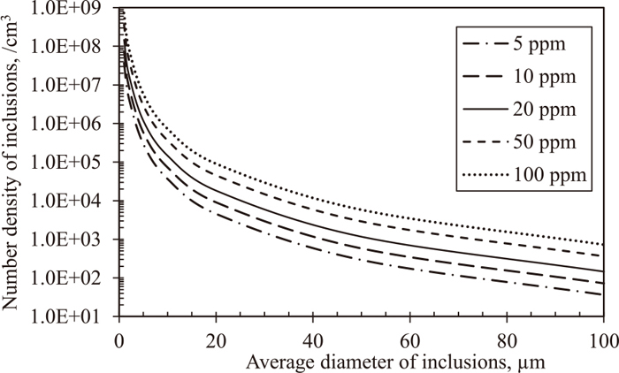
Number density of inclusions as function of total oxygen and average inclusion diameter.

The PSD of inclusions in steel is found to have a lognormal form.^24,25) The peak value of the inclusion diameter appears in the diameter of less than 10 μm.^26,27,28) The concentration of the inclusion in steel is in between 10⁵ and 10⁷ cm⁻³ (10⁵ and 10¹¹ m⁻³), when the inclusions are assumed to be 10 μm. It may be up to 10⁹ cm⁻³ (10¹³ m⁻³) before refining when the total oxygen is high.

3.2. PSD of Inclusions

In this study, three types PSD are analyzed in order to investigate their influence of PSD on the stereological methods. The simplest case is a mono dispersed particle system. The inclusion diameter as defined as 5 μm and 10 μm; while the total oxygen varies from 10 to 100 ppm. The measurement of the 2D PND is validated in a series of cases, the details of which is discussed below.

Secondly, a system containing lognormal size distributed inclusions is modeled, which is the most realistic case of inclusions in steel.^24,25) The lognormal distribution is given by   

$$f(D)=\frac{1}{{\sigma }_1\sqrt{2\pi }}exp\left(\frac{{\left(lnD-{\mu }_1\right)}^2}{2{\sigma }_1^2}\right)$$(13)

Where, D is the diameter of the 3D particles, μ₁ and σ₁ are the mean and standard deviation of the lognormal distribution.

A system containing normal size distributed inclusions is simulated for a reference to investigate the influence of PSD on the reliability of SS and MSS methods.   

$$f(D)=\frac{1}{{\sigma }_2\sqrt{2\pi }}exp\left(\frac{{\left(D-{\mu }_2\right)}^2}{2{\sigma }_2^2}\right)$$(14)

Where, D is the diameter of the 3D particles; μ₂ and σ₂ are the mean and standard deviation of the normal distribution.

3.3. Particle Dispersion

In order to validate the reliability of the stereological method, a number of 3D particles with a predefined PSD are dispersed randomly in a 3D space. A test plane is then inserted into the 3D space randomly to obtain the 2D PSD in the CS. The model of particle dispersion follows the procedures,

(1) A series of random numbers are generated randomly following the predefined PSD, which are used as the diameters of particles.

(2) A particle with a diameter from step 1 is released into the 3D space in a random position.

(3) The overlapping is avoid by calculate the central distance and the radius of every two particles in the system. A new position is generated for the latest particle until it does not overlap with any other particles. Then step 2 and 3 is repeated.

(4) A test plane at random position Z is inserted into the 3D space; and the 2D PSD and PND are measured in the test plane.

In this study, the size of the simulated 3D space is 1×1×1 cm³, which is close to a normal polished steel sample. Figure 2 gives an example of 3D space containing random dispersed particles. Due to the small size of particles and resolution limitation, the space shown in Fig. 2 is subtracted from the simulated space, which is 1 mm³ of volume.

Fig. 2.

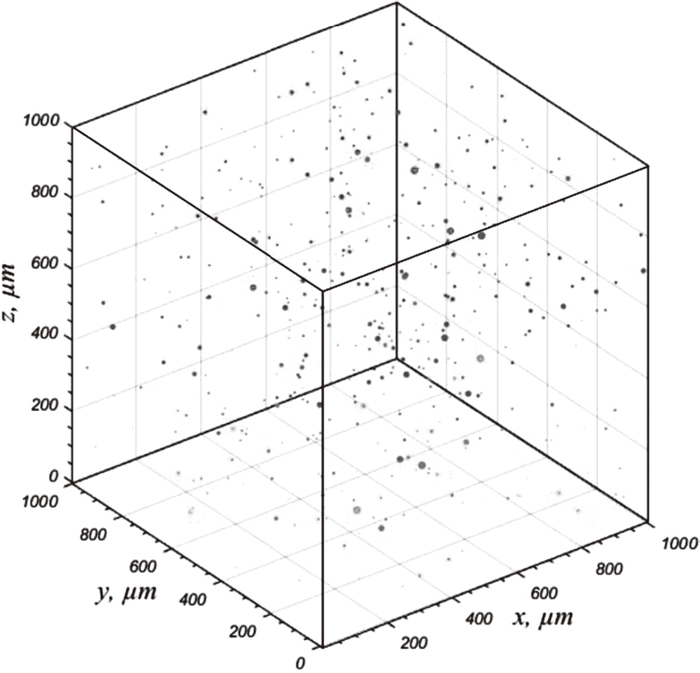
Particles dispersed in a 3D space (lognormal distribution).

4. Results and Discussion

4.1. Mono Sized Spherical Particles

Table 1 shows the assumed cases of steel samples containing mono dispersed inclusions. A number of mono sized spherical particles are dispersed randomly in the 3D space (1 cm³), whose number density and diameters are N_v and D respectively. A hundred of CS are randomly generated in the 3D space to obtain the 2D information of the inclusion particles; the area of each cross-section is corresponding to 1 cm². The measured 2D PND (N_a), area fraction (Area %), and 2D diameters (d_max and d_ave) of inclusion particles in the 2D CS are based on measurement in all the 100 random CS. The 3D PND (N_v) and 2D PND (N_a) follow Eq. (1); thus the theoretical N_a is calculated from the N_v and D by Eq. (1). On the other hand, N_v is calculated reversely from the measured 2D PND (N_a) by using the maximum (d_max) and average (d_ave) diameter in the 2D CS. The 3D PND is over estimated by using the average measured 2D diameter (d_ave), which is skewed to be a smaller value than the maximum one (d_max=D).

Table 1. Cases of steel samples with mono dispersed inclusions.

Case	A	B	C	D	E	F
D, μm	5			10
T[O], ppm	10	50	100	10	50	100
Nv, cm−3	5.83×105	2.91×106	5.83×106	7.28×104	3.64×105	7.28×105
Nv, m−3	5.83×1011	2.91×1012	5.83×1012	7.28×1010	3.64×1011	7.28×1011
Volume %	0.0038	0.0191	0.0381	0.0038	0.0191	0.0381
Meaured Area %	0.0038	0.0190	0.0381	0.0038	0.0188	0.0380
Theoritical Na, cm−2	291	1457	2913	73	364	728
Measured Na, cm−2	291	1453	2916	73	361	728
Maximum dmax, μm	5.00	5.00	5.00	10.00	10.00	10.00
Average dave, μm	3.92	3.75	6.09	6.09	7.09	7.17
Nv, cm−3 (by dmax)	5.82×105	2.91×106	5.83×106	7.32×104	3.61×105	7.28×105
Nv, cm−3 (by dave)	7.42×105	3.88×106	4.79×106	1.20×105	5.09×105	1.01×105

Figure 3 shows the measured 2D PND on each cross-section and the average value of the first n CS. The deviations of 2D PND from the average value is quite small and stable. Figure 4 shows the relative errors of 2D PND, which is calculated by the relative difference between the average 2D PND of the first n CS and the theoretical N_a in Table 1. The relative errors are significantly reduced when the number of measured CS reaches 30 in case A–C, and 20 in cases D–F. Though the errors in cases D–F is relatively larger than that of case A–C, they are still acceptable for the inclusion statistics. It is obvious that the relative errors in case A is larger than cases B and C, particularly when the measured CS are less than 30; so does case D comparing with cases E and F. It is turned out that the relative errors increases with the increasing inclusion size. The increasing errors may come from the decreasing PND because the total volume of inclusion is fixed at a certain total oxygen. It requires a larger number of measurements to achieve a random analysis when the PND of inclusions is lower.

Fig. 3.

Number density of inclusion particles on 2D CS.

Fig. 4.

Relative errors of measured inclusions number density in 2D CS.

4.2. Lognormal Distribution

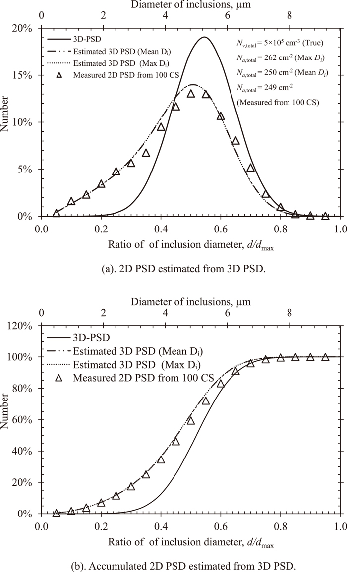
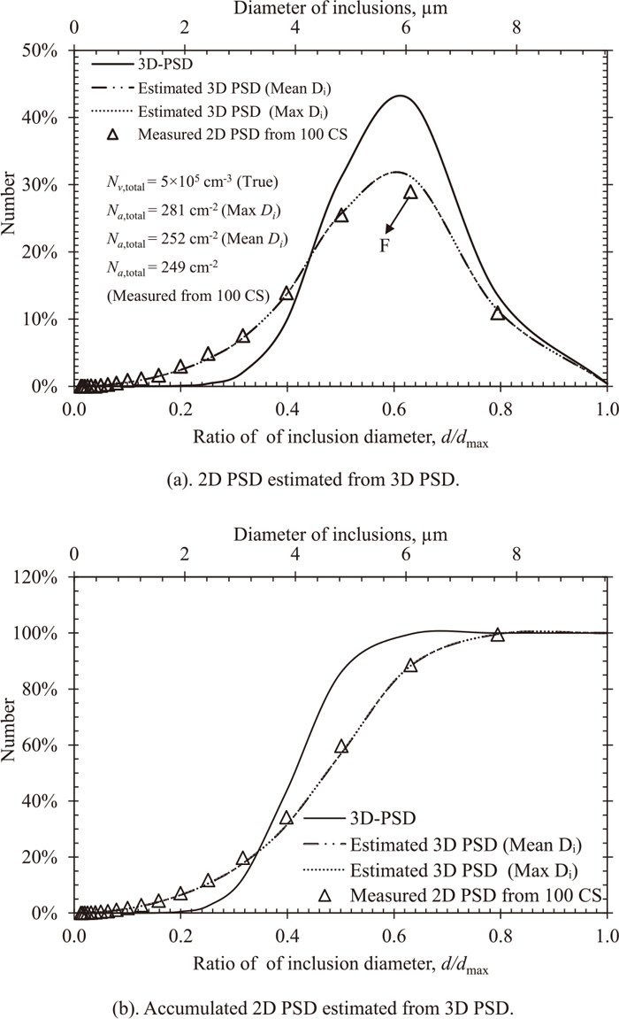
On basis of the investigation on the monodispersed inclusions above, the 3D PND in the system containing lognormal distributed particles is set as 5×10⁵ cm⁻³, which is comparable to the mono dispersed cases. The mean (μ₁) and sigma (σ₁) for the lognormal distribution in Eq. (13) is set as ln(5) μm and 0.1 that yield a series of random diameter D with mean value of 5 μm. Figure 5(a) shows the 3D PSD and the translation from 3D PSD to 2D PSD by using the SS method. Figure 5(b) shows the accumulated 3D and 2D PSD. The 3D PSD is predefined following the lognormal distribution in Eq. (13). The 2D PSD is estimated by using two different types of representative diameters of the discretized groups, maximum D_i and mean D_i. As seen in Figs. 5(a) and 5(b), the 2D PSDs translated by SS method are very close even using different representative group diameters. The estimated 2D PSD in the first group deviates from the measured value by around 5%. The 2D PND is overestimated when using the maximum D_i as the representative group diameter; while the estimation using mean D_i agrees well to the measured 2D PND.

Fig. 5.

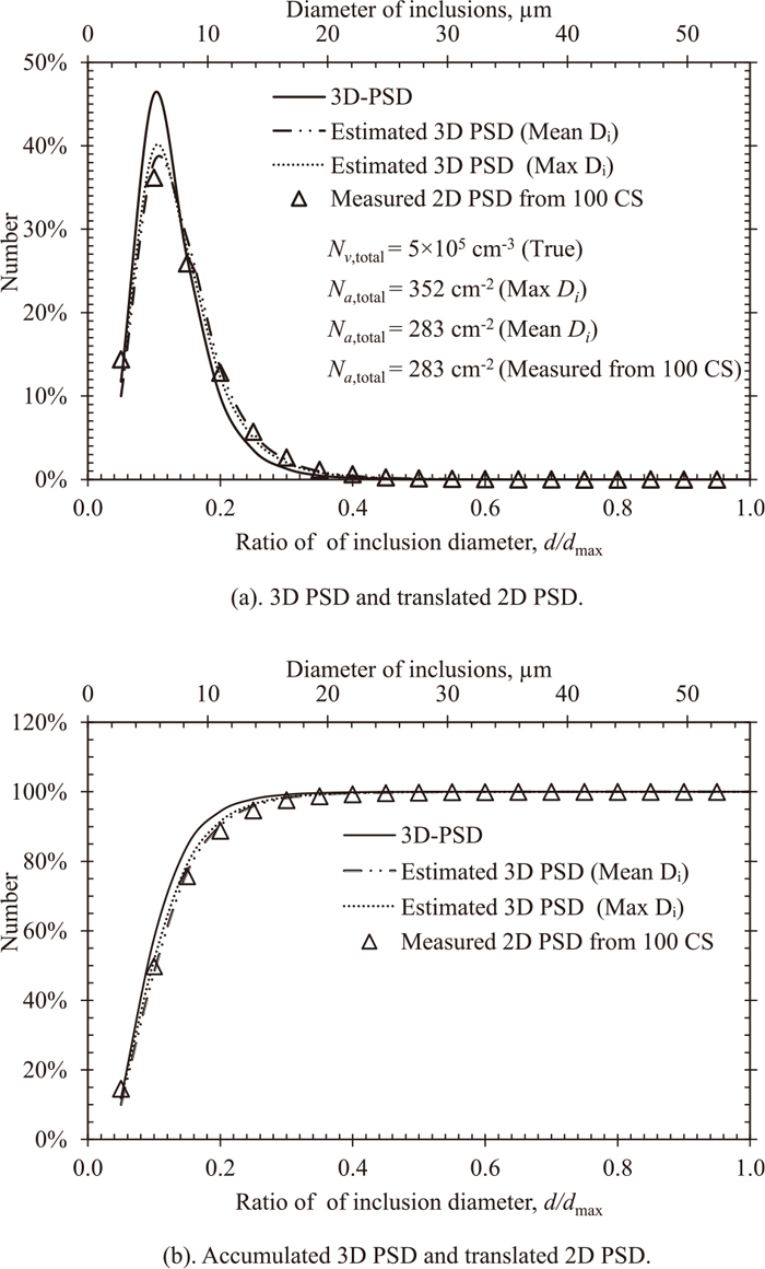
Translation from 3D PSD to 2D PSD by SS method (lognormal distribution).

Figure 6 shows the translation from 3D PSD to 2D PSD by MSS method. The 2D PSD estimated by using maximum and mean D_i are exactly overlapped. It means that the representative group diameters have no influence on the translated 2D PSDs. The estimated 2D PSD agrees very well with the measured 2D PSD in the 100 CS, which achieves a better agreement than the results from SS method. Similar to the SS method, the 2D PND is overestimated by using upper limit (maximum D_i) as the representative group diameter; while the estimated 2D PND agrees well with the measured results when the representative group diameter is set to be the mean diameter in each group.

Fig. 6.

Translation from 3D PSD to 2D PSD by MSS method (lognormal distribution).

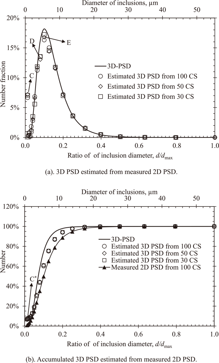
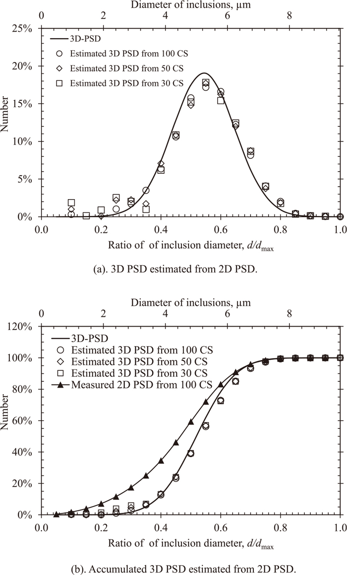
However, the translation from 3D PSD to 2D PSD is only for the sake of model validation, rather than providing practical solutions for inclusion statistics, since the 3D inclusion size distribution and number density are practically unknown. The translation from measured 2D PSD to 3D PSD attracts more interests, which are shown in Fig. 7 by using SS method. The number fractions of 3D PSD at point A is overestimated by around 9%; and it is underestimated by around 7% at point B in Fig. 7(a). Thus, the accumulated 3D PSD estimated from measured 2D PSD is overestimated at the A^* and is pulled back to fit the predefined curve of 3D PSD after point B^* in Fig. 7(b). The errors estimated 3D PSD (lognormal distribution) by SS method mostly appears in at points A^* and B^*. The minimum measured number of CS is 30, which is to guarantee the accuracy of the measurement on basis of the results drawn in the analysis of the mono distributed particle system. No significant deviations in the estimated 3D PSD are brought out by using 2D PSD measured from 30, 50, and 100 CS. Therefore, the measurement of 30 CS is quite enough to guarantee the accuracy of the inclusion statistics in steel.

Fig. 7.

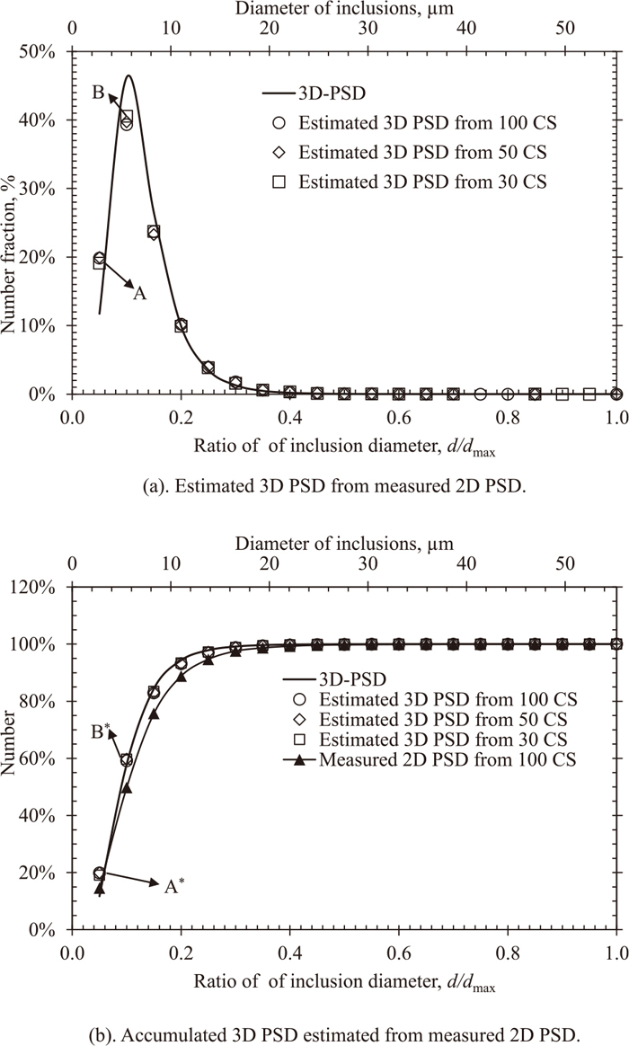
Translation from 2D PSD to 3D PSD by SS method (lognormal distribution).

As seen in Fig. 5(a), the measured number fraction in the 2D PSD is close to 40% at the peak. It is to say that most of the inclusions are sorted into the few groups with small diameter. The difference in the number fraction is too large among groups, which makes the estimation of 3D PSD (lognormal distribution) too sensitive to the slight errors of the measuring 2D PSD.

When it comes to the translation from 2D PSD to 3D PSD using MMS method shown in Fig. 8. The number fraction of inclusions in the group at point C is 7% overestimated, as seen in Fig. 8(a). While it is underestimated at points D and E by around 2%, which are acceptable errors. On the other hand, as seen in Fig. 8(b), it seems that the accumulated 3D PSD does not fit well with the predefined curve. Nevertheless, all the errors are actually from point C* with an overestimated number fraction; and the following points are underestimated to guarantee the total number fraction to be 100% in Fig. 8(b). Recall Figs. 5 and 6, the maximum number fraction of inclusions in the measured 2D PSD come out with 15% by using MSS method in Fig. 6(a), which is much smaller than that from SS method with 40% in Fig. 5(a). The number fractions in the estimated 3D PSD in Fig. 8(a) is much more even than that from SS method in Fig. 7(a). The errors of estimated 3D PSD by using MSS method are much smaller than those from SS method, except the error at point C in Fig. 8(a).

Fig. 8.

Translation from 2D PSD to 3D PSD by MSS method (lognormal distribution).

Figure 9 shows the estimated 3D PND (N_v) and the relative errors as a function of number of measured CS and representative group diameters by using SS method. The 3D PND is predefined as 5×10⁵ cm⁻³ in the simulation model. It is turned out that the N_v is underestimated when the maximum D_i in each group i is used as the representative group diameter; while the N_v is overestimated when the mean D_i represents the group diameters. The relative errors in the two ways are around 15%–20%, which is too larger to be acceptable.

Fig. 9.

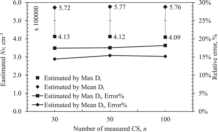
Estimated Nv and the relative errors by SS method (lognormal distribution).

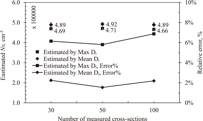
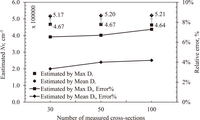
Figure 10 shows the estimated 3D PND from the measured 2D PSD and PND by using MSS method. Similar to those conclude from SS method in Fig. 9. The 2D PND is overestimated by using maximum D_i and underestimated by using mean D_i. However, the relative errors is reduced into around 6%–8% that are acceptable for inclusion statistics. Therefore, for a 3D PSD with lognormal distribution, the MSS method should be in the first place to estimate the 3D PND and PSD. The difference of errors by using the SS and modified SS methods may come from the different ways of group discretization.

Fig. 10.

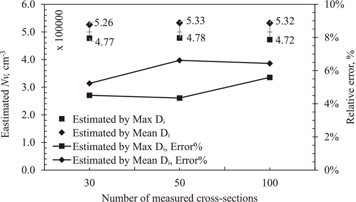
Estimated Nv and its relative errors by MSS method (lognormal distribution).

On basis of the results in Figs. 9 and 10, there is no evidence to reduce the relative errors of estimated N_v by increasing the number of measured CS for obtaining 2D PSD. It proofs again that the measurement of 30 CS is good enough to predict the 3D PSD and PND with acceptable statistical errors.

4.3. Normal Distribution

Though the lognormal distribution is most realistic for inclusions in steel, a system containing normal distributed particles is simulated as a reference, which is aiming to investigate the influence of different predefined 3D PSDs on the reliability of SS and MSS methods. The validation of the transformation from 3D PSD to 2D PSD is shown in Fig. 11. As concluded above, the representive group diameters does not lead to any difference of the translated 2D PSD from 3D PSD; while a more accurate estimated 2D PND is achieved by using the mean diameter in each group as the represent group diameter. However, the estimated 2D PSD deviates a bit from the meausred results. It is because the particles with normal distribution are sorted much more evenly into most of the groups. The errors of measurement is also evenly distributed into all the gorups that lead to the apprant small errors in each group in the 2D PSD, which can be ignored for the inclusion statistics. The errors in Fig. 11 are much smaller than those in Fig. 5 which show the 2D PSD estimated by SS method from a 3D PSD with lognormal distribution. Particularly at the point of the first group, the errors in the Fig. 5(a) is close 5%; while the deviations of the calculated and measured 2D PSD are quite small (maximum 1–2% in some groups). Therefore, to reduce the errors, the SS method should be used to calculate the 2D PSD when the 3D PSD is normal distribution. The estimated 2D PNDs by using the different representative group diameters have the same tendency to those results above.

Fig. 11.

Translation from 3D PSD to 2D PSD by SS method (normal distribution).

The translation from 3D PSD to 2D PSD by MSS method is shown in Fig. 12. A relative large deviation appears at point F Fig. 12(a); while the accuracy is acceptable for the inclusion statistics. Both SS and MSS methods deliver good estimation of 2D PSD from 3D PSD with normal distribution. Moreover, the estimated 2D PSDs achieves good agreements by using MSS method from both lognormal and normal 3D PSD. It can be concluded that the translation from 3D PSD to 2D PSD by using MSS method is independent of the predefined 3D PSD.

Fig. 12.

Translation from 3D PSD to 2D PSD by MSS method (normal distribution).

Figure 13 shows the 3D PSD (normal distribution) estimated from the measured 2D PSD by SS method. Though fluctuations appear in the first several groups with small d/d_max, the deviations are quite small (< 2%) and can be ignored in the inclusion statistics. The deviations between the estimated 3D PSD and the predefined 3D PSD are much less than those shown in Fig. 7(a), particularly in the first several groups. It is apparent that the SS method gives a better estimation of the 3D PSD with a normal distribution than the 3D PSD with a lognormal distribution.

Fig. 13.

Translation from 2D PSD to 3D PSD by SS method (normal distribution).

Figure 14 shows the estimated 3D PSD from the measured 2D PSD by using MSS method for a normal distributed particle system. Comparing with Fig. 8 (MSS method for lognormal 3D PSD), more fluctuations appear in the first a few groups with small d/d_max; and a large deviation appears at point G in Fig. 14(a). The deviations at points H and K in Fig. 14(b) are too large to be accepted. Therefore, The MSS method could not give a good prediction of the 3D PSD from measured 2D PSD for a system containing normal distributed particles; while it is a good choice for the system containing lognormal distributed particles. Thus, SS method achieves a higher accuracy to predict the 2D PSD from a 3D PSD with normal distribution; while MSS method is better for a system containing lognormal distributed particles.

Fig. 14.

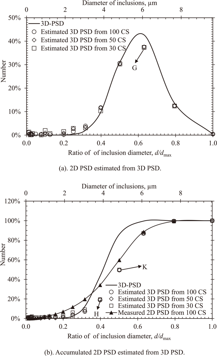
Translation from 2D PSD to 3D PSD by MSS method (normal distribution).

Concerning the estimated 3D PND, the results are shown in Figs. 15 and 16. When the predefined 3D PSD is a normal distribution, 3D PNDs from the SS method are underestimated by using both maximum and mean D_i as representative group diameters. The estimated 3D PND has a higher accuracy when the mean D_i is used as the representative group diameter, which is same as that concluded in all the estimation of 3D PNDs above. Furthermore, for a system containing normal distributed 3D particles, the SS method achieves a slight higher accuracy than MSS method, though all of the relative errors are less than 8% and acceptable. Therefore, it gives more credit to the SS method for the translation between 3D and 2D PSD and PND.

Fig. 15.

Estimated 3D PND by SS method (normal distribution).

Fig. 16.

Estimated 3D PND by MSS method (normal distribution).

5. Conclusions

In this study, we developed a model to disperse series of 3D particles with a certain PSD into a space. The reliability of SS and MSS methods on inclusion statistics are investigated by the developed simulation model. Three type of PSDs are calculated to clarify their influence on the reliability of the stereological models. The spherical particle systems are used in this study, which is a simplified model of inclusions in steel.

(1) In a system containing monodisperse particles, the fluctuations of the measured 2D PND in the CS are quite small and stable. The average 2D PND is reliable from a measurement of 30 CS.

(2) Both SS and MSS methods deliver good estimation of 2D PSD from 3D PSD with normal distribution; while the translation from 3D PSD to 2D PSD by using MSS method is independent of the types of the predefined 3D PSD.

(3) The MSS method should be put into the first place when estimating the 3D PSD from the measured 2D PSD, when the 3D PSD is a lognormal distribution; while the SS method should be used when the 3D PSD is a normal distribution.

(4) The representative group diameter has no influence on the translated 2D PSD from the 3D PSD, which is also independent of the types of 3D PSD. The 2D PND is overestimated when the maximum D_i is used as the representative group diameter; while it agrees well with the measured 2D PND when the mean D_i is in use.

(5) The estimation of 3D PND is more reliable by using mean D_i as the representative group diameter. The MSS method achieves a higher accuracy than SS method to estimate the 3D PND for a 3D PSD with lognormal distribution; while SS method is better when the 3D PSD is a normal distribution.

Acknowledgements

This work was supported in part by a Grant-in-Aid for Scientific Research (A) (No. 22246097) provided by the Japan Society for the Promotion of Science (JSPS).

References

• 1)   K. W.  Lange: Int. Mater. Rev., 33 (1988), 53.
• 2)   W. B.  Morrison: Ironmaking Steelmaking, 16 (1989), 123.
• 3)   L. F.  Zhang and  B. G.  Thomas: ISIJ Int., 43 (2003), 271.
• 4)   S.  Taniguchi,  A.  Kikuchi,  T.  Ise and  N.  Shoji: ISIJ Int., 36 (1996), S117.
• 5)   T.  Nakaoka,  S.  Taniguchi,  K.  Matsumoto and  S. T.  Johansen: ISIJ Int., 41 (2001), 1103.
• 6)   T.  Li,  S.  Shimasaki,  S.  Taniguchi and  K.  Uesugi: 13th Int. Conf. Aluminum Alloys, TMS, Warrendale, PA, (2012), 1337.
• 7)   T.  Li,  R.  Oka,  S.  Taniguchi and  S.  Shimasaki: CAMP-ISIJ, 24 (2011), 811.
• 8)   H.  Arai,  K.  Matsumoto,  S.  Shimasaki and  S.  Taniguchi: ISIJ Int., 49 (2009), 965.
• 9)   T.  Li,  S.  Shimasaki,  S.  Taniguchi,  S.  Narita and  K.  Uesugi: ISIJ Int., 53 (2013), 1958.
• 10)   L.  Zhang and  B. G.  Thomas: ISIJ Int., 43 (2003), 271.
• 11)   H. A.  Schwartz: Met. Alloys, 5 (1934), 139.
• 12)   S. A.  Saltykov: Stereometric Metallography, 2nd ed., Metallurgizdat, Moscow, (1958), 81.
• 13)   E.  Scheil: Z. Anorg. Allg. Chem., 201 (1931), 259.
• 14)   E.  Scheil: Z. Metallkd., 27 (1935), 199.
• 15)   S. A.  Saltykov: Stereology: Proc. 2nd Int. Cong. for Stereology, ed. by H. Elias, Springer-Verlag, New York, (1967), 163.
• 16)   M.  Enomoto and  Y.  Kobayashi: ISIJ Int., 39 (1999), 600.
• 17)   D. F.  Susan,  J. D.  Puskar,  J. A.  Brooks and  C. V.  Robino: Proc. 11th Solid Freeform Fabrication Conf., Austin, TX, (2000), 50.
• 18)   T.  Li,  S.  Shimasaki,  S.  Taniguchi,  S.  Narita and  K.  Uesugi: ISIJ Int., 53 (2013), 1943.
• 19)   T.  Li,  S.  Shimasaki,  S.  Taniguchi,  S.  Narita and  K.  Uesugi: CAMP-ISIJ, 17 (2012), 985, CD-ROM.
• 20)   J.  Takahashi and  H.  Suito: Acta Mater., 49 (2001), 711.
• 21)   J.  Takahashi and  H.  Suito: Mater. Sci. Technol., 18 (2002), 103.
• 22)   J.  Takahashi and  H.  Suito: Metall. Mater. Trans. A, 34A (2003), 171.
• 23)   R. T.  Dehoff: Quantitative Microscoy, ed. by R. T. Dehoff and F. N. Rhines, Mcgraw-Hill, New York, (1968), 149.
• 24)   C. W.  Anderson,  G.  Shi,  H. V.  Atkinson and  C. M.  Sellars: Acta Mater., 48 (2000), 4235.
• 25)   H. V.  Atkinson and  G.  Shi: Prog. Mater. Sci., 48 (2003), 457.
• 26)   L.  Huet,  P.  Jonsson and  F.  Reinholdsson: Steel Times Int., 21 (1997), 47.
• 27)   H.  Matsuta,  T.  Sato and  M.  Oku: ISIJ Int., 36 (1996), S125.
• 28)   M.  Kawakami,  T.  Nishimura,  T.  Takenaka and  S.  Yokoya: ISIJ Int., 39 (1999), 164.