Intermediate-angle Neutron Scattering Instrument for Quantitative and Non-destructive Characterization of Nanostructures in Steels and Other Alloys

Abstract

For characterizing nanostructures embedded in a metallic matrix, a newly designed intermediate-angle neutron scattering (iANS: “irons”) instrument has been developed that shortens the distance between the sample and detector and is combined with a time-of-flight (TOF) technique. Since the momentum transfer (Q) resolution can be relaxed to provide an optimum Q-range when we focus on characterizing nanoscale heterogeneity, a much higher neutron flux can be utilized for the measurements than those available in a conventional small-angle neutron scattering (SANS) instrument. Consequently, iANS gives sufficiently high quality profiles for quantitative analysis on an absolute unit scale even using a compact accelerator driven neutron source (CANS). The results obtained at the Hokkaido University Neutron Source (HUNS) are compared to those obtained in large facilities. Some results obtained by iANS, are compared to those obtained by small angle X-ray scattering (SAXS) with respect to SAXS/SANS contrast variation.

1. Introduction

Recent developments in high-strengthened steels generally require accurate microstructure control down to the nanoscale region. Some of them are already in a mass-production state, typically represented by nano-HITEN type steels.¹⁾ Dispersion strengthening including precipitation hardening is sensitive to the number density and size of the dispersed particles (i.e. precipitates or other heterogeneities). Therefore, characterization methods for those parameters are important to control the quality of the products and further the development of high performance steels. Important features required in the analysis include the following; accuracy of “size and number density” evaluation, “determination of phase and composition of the heterogeneities” and “simple preparation process”. Transmission electron microscopy (TEM) satisfies most of these requirements except for the difficulty in sample preparations and statistical analysing processing.²⁾ Since atom probe tomography (APT) gives detailed information of the partitioning of each element, it is extremely powerful for understanding the mechanism of the formation of nanoscale heterogeneities.³⁾ However, it is difficult to obtain average features due to the limitation of measured volume. The calculation phase diagram (CALPHAD) technique provides good guidance and good predictions for the total amount of heterogeneities formed in the system and it may be possible to predict microstructures by combining it with the phase-field method.⁴⁾ However, it is sometimes difficult to apply to the industrial products due to the complex compositions and processes involved.

While the use of the small-angle scattering (SAS) technique alone cannot determine the phase and composition, it can easily give statistically representative values for average size and number densities of the heterogeneities. Using the features of SAS, the application to Fe–Cu alloys has been reported by Osamura et al. using SANS^5,6) and Deschamps et al. by SAXS.⁷⁾ Deschamps et al. also reported detailed analysis of the microstructure evolution of Al alloys by time-resolved SAXS.^8,9,10) Odetta et al. reported detailed microstructural analysis of oxide dispersed strengthened (ODS) steels using a combination of SANS, ATP and TEM.^11,12) SANS studies of nanoscale carbides such as TiC,¹³⁾ NbC¹⁴⁾ and VC¹⁵⁾ has been reported by different groups. In addition to these basic SAS applications, one of the authors (MO) proposed a new way to determine phase by the combining SANS and SAXS methods. This technique, known as the alloy contrast variation (ACV) method,¹⁶⁾ utilizes the scattering length difference of each element between X-rays and neutrons. In addition to phase determination, it can give information about the composition of the heterogeneities embedded in the matrix. Applying ACV, it has been confirmed that oxide in ODS steels are free from Fe.¹⁶⁾ For the V added steels, Oba et al. reported that nanoscale VC has off-stoichiometry in the early stage of precipitation.¹⁵⁾ Coakley et al. reported partitioning of constituent elements to nanoscale ω precipitation in the titanium alloys.¹⁷⁾ As these examples show, the ACV technique is particularly useful when partitioning of the main constituent element occurs. For example, in the case of steels, the Fe content in heterogeneities that are less than 5 nm in size cannot be investigated by other techniques without the effects of smearing by the surrounding Fe in the matrix. Therefore, expanding the applications of ACV to other steels and alloys may bring about new knowledge concerning the mechanism of the formation of nanoscale heterogeneities and also their effects on the alloy properties. Thanks to the recent development of an X-ray mirror and a micro-focus source, it is possible to perform nanostructure-characterizations using laboratory SAXS,^15,16,17) while the opportunity to use SANS is still limited due to the shortage of SANS instruments. Regular SANS instruments are about 20 to 40 m length and therefore, two or three SANS instruments are the maximum number available at each neutron source. The number of neutron source, as we know, is also very limited. In Japan only two facilities are open for users from industry, i.e. the JRR-3 research reactor (suspended till 2018 (expected)) and the Japan Proton Accelerator Research Complex (J-PARC). Thus, developing a compact SANS which can be multiply installed in large scale facilities and/or can be used as the instrument with a compact accelerator driven neutron source (CANS), is expected to overcome the present limitation.

We also emphasize the point that the SANS technique can be the easiest among many techniques to apply to nanostructure-characterization, especially for steel research, due to the simple sample preparation. For SANS measurements, sample preparation includes only cutting into the proper size, typically about 10–20 mm square and 1–2 mm thickness. It is probably easier than the sample preparations for optical microscope (OM) observations because SANS does not require a mirror-like surface. Thus, our target is to develop a new intermediate-angle neutron scattering instrument “iANS” which is usable with a CANS, and prove that the data obtained by iANS is at a comparable level to that obtained in standard facilities in order to promote detailed discussion of the partitioning of main elements and increasing the speed of nanostructure-characterization.

2. Experimental

2.1. Basic Design Concept of iANS for Characterizing Nanoscale Heterogeneities

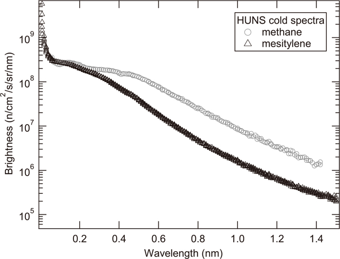
Compared to the neutron flux of large facilities, typically about 10⁸ neutrons/cm²/s, that of CANS is usually 4 orders smaller, at a level of 10⁴ to 10⁵ neutrons/cm²/s. Table 1 and Fig. 1 shows the performance of the cold neutron source at the Hokkaido University Neutron Source (HUNS). Clearly, we cannot expect a CANS instrument to perform at this level. Instead, some special strategies are required to achieve competitive performance to those in big facilities. Most regular SANS systems are designed for low-Q observations, which is typically shown by the fact that the performance of SANS is often expressed by the minimum Q, Q_min, measured by each instrument. Here, Q is the momentum transfer and defined as Q = 4πsinθ/λ (2θ: scattering angle, λ: wavelength of neutron or X-ray). However, in metallurgy, we have many tools for characterizing from the micron scale to a few ten nanometers, such as OM, a mapping technique combined with scanning electron microscope (SEM) or TEM, and chemical extraction residues.¹⁸⁾ In contrast, the choice of characterization methods is limited to TEM and/or APT when the size of heterogeneities reaches to a few nanometers. Therefore, the target of the new iANS instrument is to observe the Q-range from 0.2 to 10 nm⁻¹, a region whose usefulness has been already shown by laboratory SAXS measurements.^15,16,17) It is advantageous that instruments at CANS can be optimized from source to the detector for this fixed purpose.

Table 1. List of important parameters of the cold source at HUNS.

Frequency	50 Hz
Accelerating Voltage	34 MeV
Beam current	34 μA (3 μsec width)
Beam Power	1.16 kW
Moderator	coupled 40 K solid methane or mesitylene
Moderator size (Beam size at moderator surface)	12 cm × 12 cm × 5 cm (10 cm × 10 cm)
Integrated Neutron Flux at 6 m (≦ 0.5 eV)	104 n/cm2/s
Cold Neutron Flux (at sample position)	103 n/cm2/s

Fig. 1.

The performance of the cold neutron source at HUNS, for methane (circle) and for mesitylene (triangle).

One of the keys for SANS measurements of alloys is to suppress the double Bragg diffraction effects which are shown in the results section. For this purpose, the wavelengths which are used for SANS analysis should be two times larger than maximum lattice plane spacing d_max (2d_max = 2d₁₁₀ = 0.405 nm for the ferritic steels). For TOF measurements with such large wavelength, the efficiency of the usage neutron is higher when the total length of the instrument is shorter because it is possible to prevent frame overlap.¹⁹⁾

Another, and most important key point is to optimize the Q-resolution for increasing the usage of neutrons. When the Q-resolution is relaxed, we can permit the introduction of neutrons with larger divergence than those when employing the regular Q-resolution of SANS. In general, the Q resolution is defined as ΔQ/Q, where ΔQ is the FWHM value in the case of a Gaussian distribution. Because the measured detector count rate C_D is roughly proportional to the fourth power of ΔQ,²⁰⁾ the gained flux can be expressed as follows.   

$$C_{\text{D}}\propto \mathrm{\Delta }{Q}^4$$(1)

Since some other effects are ignored for simplification, C_D tends to be overestimated by Eq. (1). However the order of the C_D is still reasonable. If we set the Q resolution to ΔQ/Q= 30%, then ΔQ= 0.06 nm⁻¹ at Q_min = 0.2 nm⁻¹ is required for iANS optics, while ΔQ= 0.009 nm⁻¹ at Q_min = 0.03 nm⁻¹ is needed for regular SANS instruments. Consequently, the C_D of iANS is at most (0.06/0.009)⁴ = 2000 times higher than that of a regular SANS system. Under these considerations, the optimum design was determined as shown in Fig. 2 and the parameters used are listed in Table 2.

Fig. 2.

Schematic drawing of the iANS at HUNS. Corresponding instrument parameters are explained in Table 2. (Online version in color.)

Table 2. List of important parameters of the iANS instrument at HUNS.

Qmin	0.25 nm−1
Qmax	6.5 nm−1 (non crystalline: 50 nm−1)
Available Wavelength	0.07–1.3 nm (200 channels, Δt = 100 μsec)
Detector Area	600 mm × 200 mm
Detector element size	5 mm × 12.7 mm
Detector type	0.5 inch3He PSD (600 mm effective length)
L1 (source to sample length)	5500 mm
L2 (sample to detector length)	500 mm
d1 (1st pinhole diameter: moderator size)	100 mm
d2 (sample size)	φ10 or φ13 mm
Shielding and Collimator material	Cd + boric acid resin
Sample environment	Vacuum

Another important requirement for ferritic steels is applying a magnetic field which can saturate the magnetization for separating the intensity into the magnetic and nuclear components.²¹⁾ While an electromagnet is usually used for this purpose,²²⁾ it would be too large to be installed in an iANS system. Therefore, a sample holder with NdFeB permanent magnets specially designed by TOWA Co., Ltd.²³⁾ (Fig. 3) is used for iANS. Based on our experience, the field larger than 0.5 T is enough for saturating magnetization of ferritic steels in general,²¹⁾ while the steel with severe deformation is recommended to be measured in higher fields. A sufficiently uniform magnetic field of 0.6 T can be applied to the area irradiated by neutrons, typically in the range of 10–13 mm in diameter.

Fig. 3.

Exterior of NdFeB permanent magnet with sample holder designed for iANS. (Online version in color.)

2.2. Data Reduction

Because of the background produced by the SANS optics themselves, data reduction is required for obtaining the scattering from the samples. For a fixed wavelength, the reduction is done using the following equations.   

$$\frac{d\mathrm{\Sigma }}{d\mathrm{\Omega }}\left(Q\right)=\frac{i_{\text{s}}\left(Q\right)}{d\hspace{0.17em}S\hspace{0.17em}\eta \hspace{0.17em}{\phi }_0\mathrm{\Delta }\mathrm{\Omega }}$$(2)

  

$$\begin{array}{l}{i}_{\text{s}}\left(Q\right)=\frac{1}{T{r}_{\text{s}+\text{c}}}\left(\frac{I_{\text{s}+\text{c}}\left(Q\right)}{t_{\text{s}+\text{c}}}-\frac{I_{\text{b}}\left(Q\right)}{t_{\text{b}}}\right)\\ \hspace{1em}\hspace{1em}\hspace{0.5em}-\frac{1}{T{r}_{\text{c}}}\left(\frac{I_{\text{c}}\left(Q\right)}{t_{\text{c}}}-\frac{I_{\text{b}}\left(Q\right)}{t_{\text{b}}}\right)\end{array}$$(3)

Here, Tr_s+c is the transmission of the “sample and cell” (if nothing except sample is in the beam line, it corresponds to the transmission of the “sample”) and Tr_c is transmission of the cell (it is unity for the above parenthetical case), I is the observed intensity and t is the measurement time of “sample and cell”, cell and blocked beam (corresponding subscription is s+c, c and b, respectively). The quantities S, η and φ₀ are the beam size, the efficiency of the detector and the flux of the incident beam, respectively. The term 1/Sηφ₀ is determined by using a secondary standard, such as glassy carbon.²⁴⁾ Other quantities, d and ΔΩ are the sample thickness and the solid angle, respectively. In the TOF type measurements, η, φ₀ and Tr become the function of λ as shown in Fig. 1 for φ₀(λ) as the example. In Fig. 4, a typical transmission spectrum of ferritic steel is also shown as a function of wavelength. Therefore, Eqs. (2) and (3) for TOF measurements are expressed as follows.   

$$\frac{d\mathrm{\Sigma }}{d\mathrm{\Omega }}\left(Q\right)=\frac{i_s\left(\lambda ,\theta \right)}{d\hspace{0.17em}S\hspace{0.17em}\eta \left(\lambda \right)\hspace{0.17em}{\phi }_0\left(\lambda \right)\mathrm{\Delta }\mathrm{\Omega }}$$(2’)

  

$$\begin{array}{l}{i}_s\left(\lambda ,\theta \right)=\frac{1}{T{r}_{\text{s}+\text{c}}\left(\lambda \right)}\left(\frac{I_{\text{s}+\text{c}}\left(\lambda ,\theta \right)}{t_{\text{s}+\text{c}}}-\frac{I_{\text{b}}\left(\lambda ,\theta \right)}{t_{\text{b}}}\right)\\ \hspace{1em}\hspace{1em}\hspace{1em}\hspace{0.17em}-\frac{1}{T{r}_{\text{c}}\left(\lambda \right)}\left(\frac{I_{\text{c}}\left(\lambda ,\theta \right)}{t_{\text{c}}}-\frac{I_{\text{b}}\left(\lambda ,\theta \right)}{t_{\text{b}}}\right)\end{array}$$(3’)

Fig. 4.

A typical transmission spectrum of ferritic steel obtained by iANS.

In the TOF case, φ₀ is determined at certain wavelengths by using a secondary standard. The direct intensity is monitored by the small hole in the beam stopper during scattering measurements for determining both the shape of φ₀(λ) and the transmission Tr(λ). Therefore, it is possible to measure SANS and the Bragg edge simultaneously.²⁵⁾ Intensity data are collected three dimensionally, i.e. x, y, t of the detector positions and time of flight. All data reduction has been processed in 3D data. For transforming to one dimensional, I-Q data, home-made code for Mathematica²⁶⁾ is used. The code for Igor Pro²⁷⁾ is also available. The details of the code and theoretical approach for absolute unit correction will be explained in the following paper.²⁸⁾

2.3. Other Experimental Procedures

Some of the profiles were compared to the regular SAS instruments. Regular SANS profiles were measured on the 18M SANS instrument in the High-flux Advanced Neutron Application ReactOr (HANARO) in Korea Atomic Energy Research Institute (KAERI). The wavelength of 4.82 nm and 9.57 nm were used for obtaining a wide range of Q. All the SAXS profiles were obtained using a laboratory SAXS with a Mo-target and confocal mirror (RIGAKU NANO-Viewer).

Glassy carbon which had been calibrated in the Advanced Photon Source in Argonne National Lab., was used as the standard for absolute intensity²⁴⁾ and was also used for checking the accuracy of the wavelength collection. Silver behenate (C₂₂H₄₃AgO₂) as a standard for powder diffraction was used for calibrating Q and evaluation of the resolutions.²⁹⁾ The high nitrogen steels,³⁰⁾ Ti added steels and Al alloys (7000 series) were delivered by Daido Steel Co., Ltd., JFE Steel Corporation and Toyota Central R&D Labs., Inc., respectively. The thickness of steels for iANS measurements is 2 mm and that of Al alloy is 3.8 mm.

3. Results

3.1. Measurements of Standard Samples

Figure 5(a) show the I(Q) data of standard glassy carbon obtained by iANS for each wavelength. These data are plotted after correcting by Eqs. (2’) and (3’) and show almost identical profiles, indicating that the above wavelength correction is working properly. Figure 5(b) shows fully processed data after summing and averaging of all the profiles in Fig. 5(a) together with the data supplied with the sample. Note that the Q_min reaches to 0.25 nm⁻¹ which is close to our designed target and Q_max can reach to 50 nm⁻¹ which approaches the wide angle neutron diffraction (WAND) range.

Fig. 5.

Profiles of glassy carbon measured by iANS. (a) Each profile is obtained by choosing the range of wavelengths described in the legends. (b) The fully processed profile of glassy carbon (markers). The profile obtained by USAXS at Advanced Photon Source is also plotted (solid line) after dividing by the factor for a neutron (6.467).²³⁾ (Online version in color.)

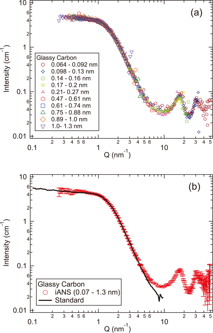
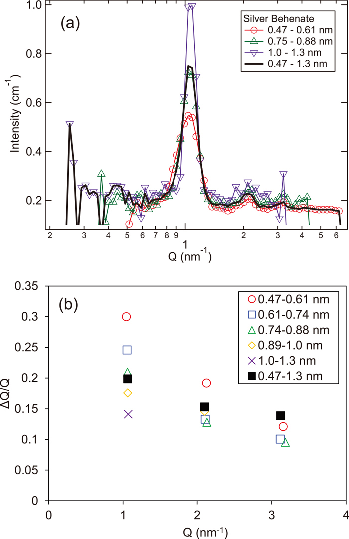
Figure 6(a) shows the profiles for silver behenate that is used for calibration of Q space and Q-resolution evaluation.²⁹⁾ The series of peaks attributed to the d spacing of 5.838 nm can be observed up to 3rd order (d₀₀₃), indicating good performance of iANS for nanoscale observation. Resolution variation is also observed due to the different scattering angle for the same Q depending on wavelength, and it broadens at short wavelengths. Although the asymmetric resolution function should be used for an accurate analysis of wavelength resolution because of the coupled-moderator feature,³¹⁾ ΔQ is obtained as the FWHM value of a Gaussian function for simplification. Figure 6(b) shows the dependence of Q resolutions, and ΔQ/Q on both wavelengths and peak positions. The evaluated resolution ΔQ/Q was close to our target value and low enough to analyse SAS profiles.

Fig. 6.

(a) Experimental data of silver behenate of iANS, reduced in the wavelength band as shown in the legends (markers) and averaged value (solid line). (b) Evaluated dependence of Q resolution at each peak measured at different wavelength. (Online version in color.)

3.2. Measurements of Steels and Other Alloys

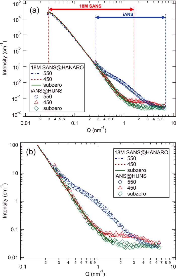
Figure 7 shows the comparison between the profiles of high nitrogen steel with different tempering temperatures obtained by 18M SANS at HANARO and by iANS. The one without tempering is featureless due to the lack of a nano-precipitate.³²⁾ After tempering at 450°C, a clear increment of SANS intensity in the high-Q region (Q ≥ 1.0 nm⁻¹) is observed. The curves obtained at HANARO cover a wide Q-range (Q = 0.03 nm⁻¹ ~1.5 nm⁻¹) as shown in Fig. 7(a). However, this is a little shortage for analysing nano-precipitates which appear as intensity changes in the Q-range higher than 1 nm⁻¹ as shown in Fig. 7(b). Since the purpose of regular SANS instruments is usually to observe lower-Q data, they have to use the conditions that is less than optimum for our purpose. The 18M SANS, for example, has the option for higher Q measurements up to 4 nm⁻¹ by using short wavelengths, but the flux at such short wavelengths is relatively low. Some of the SANS instrument is equipped with a high-Q detector which needs additional calibration. In contrast, iANS can give high-Q information in one measurement with a single detector system because the acceptance angle is large due to the short L₂ (see Table 2). Note that the absolute unit profiles shown here are obtained separately at each facility, and they perfectly coincide. The results indicate that iANS data reduction and calibration by glassy carbon²⁴⁾ is accurate for measuring on an absolute unit scale. Note that the applied magnetic field is 1.0 T for 18M SANS experiments show the same profiles with iANS indicating 0.6 T is enough for saturating.

Fig. 7.

Profiles of high nitrogen steel tempered at different temperatures, curves: measured by 18 M SANS at HANARO, markers: measured by iANS (a) full region covered by 18M SANS and iANS (b) enlarged Q region corresponding to the change caused by nanosize precipitates. All profiles measured perpendicular to the magnetic field, i.e. magnetic and nuclear scattering is presented for enhancing the small change in SANS profiles of the samples with subzero and 450°C tempering. Error bars are less than marker size. (Online version in color.)

Based on the above results, the ACV method¹⁶⁾ can work only with the iANS and labo-SAXS, i.e. both of the in-house systems on our campus. Figure 8 shows TiC precipitates in the steel and MgZn₂ precipitates in Al alloy as examples. The observed intensity ratios between SAXS and SANS are 14 (±10%) and 225 (±10%), respectively. The scattering length densities are obtained from mass densities and nominal compositions for matrices, and from lattice constants and stoichiometric compositions for precipitates.³³⁾ The expected intensity ratio yields 14.1 for TiC and 230 for MgZn₂ which are close matches with the observed values within the error. Therefore, we can conclude that evaluating composition and phase only using in-house SAS instruments is now feasible and ready for further research in any alloy systems.

Fig. 8.

Examples of ACV analysis for the Ti-added steel (circles) and the 7000 series aluminum alloy (triangles); observed intensity ratio is about 14 (±10%) and 225 (±10%), respectively. Error bars of SAXS measurements are less than marker size. (Online version in color.)

3.3. SANS Mode and WAND Mode

As often pointed out in the references, double Bragg diffraction is serious problem when we use λ less than 2d_max.³⁴⁾ Figure 9 shows the comparison of the profiles obtained using wavelengths larger, and less than, 2d_max (2d_max = 2d₁₁₀ for the ferritic steels, yields λ > 0.405 nm in ideal case, while it depends on the neutron source with different wavelength resolution). The reason why the difference appears is attributed to the larger scattering cross section than the absorption cross section of the neutron in the wavelength range below 2d_max.³⁵⁾ Therefore there is a high probability that the beam diffracted by a certain plane can return to the small angle area by double diffraction. The simple way to prevent it is by using a wavelength larger than 2d_max to avoid any Bragg diffraction. However, a beam with a wavelength less than 2d_max is useful for obtaining diffraction in the WAND region. As shown in Fig. 9 as well as Fig. 5, the Bragg peaks of each material appear. In Fig. 9, we see two peaks corresponding to d₁₁₀ and d₂₀₀ from the bcc matrix. In addition, the Bragg edge information is included in the transmission spectra, as already shown in Fig. 4. The Bragg edge was clearly observed at 0.405 nm corresponding to diffraction of d₁₁₀ and therefore, it contains information on the crystalline structure for the matrix phase.³⁶⁾ Consequently, iANS can provide a complete set of information from nanoscale precipitation to structures (ex. grain size, texture) of matrix or major phases by combining SANS, WAND and Bragg edge measurements.^25,36)

Fig. 9.

Wavelength dependence of SANS profiles. Black dotted line represent regular SANS analysis. The deviation from this profile is due to double Bragg diffraction (markers). Bragg diffraction peaks corresponding to d₁₁₀ and d₂₀₀ from the bcc matrix are observed in the WAND region (solid line). (Online version in color.)

4. Summary and Further Perspective

A newly designed intermediate Angle Scattering instrument “iANS” for non-destructive nanostructure-characterization of steels and other alloys has been developed. It provides accurate profiles of absolute intensity in the Q-range from 0.25 to 6.5 nm⁻¹ for SANS mode and 50 nm⁻¹ for WAND mode. The present results show that the accuracy in the absolute unit scale is high enough for ACV analysis. The measurement time is from 3 (solid methane moderator) to 6 hours (solid mesitylene moderator) under the present HUNS conditions. The HUNS-II now planned to replace the HUNS-I system is expected to make measurement times shorter by about one third. Taking the simple sample preparation into account, SANS can be the easiest and quickest measurement method for nanostructure analysis. Therefore, we believe that iANS with a CANS source has the potential for accelerating development of new alloys, once the CANS system has spread to a wider number of many sites.

Acknowledgement

Part of this study is supported by KAKENHI B–24360296, type 1 Research Group by ISIJ and Innovative Structural Materials Association. We thank to collaborators in Daido Steel Co., Ltd., JFE Steel Corporation and Toyota Central R&D Labs., Inc., for helping with sample preparations and fruitful discussions.

References

• 1)   Y.  Funakawa,  T.  Shiozaki,  K.  Tomita,  T.  Yamamoto and  E.  Maeda: ISIJ Int., 44 (2004), 1945.
• 2)  For example,  D. B.  Williams and  C. B.  Carter: Transmission Electron Microscopy, 2nd Ed., Springer, New York, (2009), 1.
• 3)  For example,  T. F.  Kelly and  M. K.  Miller: Rev. Sci. Instrum., 78 (2007), 031101.
• 4)  For example,  L. Q.  Chen: Annu. Rev. Mater. Sci., 32 (2002), 113.
• 5)   K.  Osamura,  H.  Okuda,  M.  Takashima,  K.  Asano and  M.  Furusaka: Mater. Trans. JIM, 34 (1993), 305.
• 6)   K.  Osamura,  H.  Okuda,  K.  Asano,  M.  Furusaka,  K.  Kishida,  F.  Kurosawa and  R.  Uemori: ISIJ Int., 34 (1994), 346.
• 7)   A.  Deschamps,  M.  Militzer and  W. J.  Poole: ISIJ Int., 43 (2003), 1826.
• 8)   A.  Deschamps,  F.  Livet and  Y.  Brèchet: Acta Mater., 47 (1999), 281.
• 9)   T.  Marlaud,  A.  Deschamps,  F.  Bley,  W.  Lefebvre and  B.  Baroux: Acta Mater., 58 (2010), 248.
• 10)   B.  Decreus,  A.  Deschamps,  F.  De Geuser,  P.  Donnadieu,  C.  Sigli and  M.  Weyland: Acta Mater., 61 (2013), 2207.
• 11)   M. J.  Alinger,  G. R.  Odette and  D. T.  Hoelzer: Acta Mater., 57 (2009), 392.
• 12)   G. R.  Odette,  M. J.  Alinger and  B. D.  Wirth: Annu. Rev. Mater. Res., 38 (2008), 471.
• 13)   H.  Yasuhara,  K.  Sato,  Y.  Toji,  M.  Ohnuma,  J.  Suzuki and  Y.  Tomota: Tetsu-to-Hagané, 96 (2010), 545 (in Japanese).
• 14)   F.  Perrard,  A.  Deschamps,  F.  Bley,  P.  Donnadieu and  P.  Maugis: J. Appl. Crystallogr., 39 (2006), 473.
• 15)   Y.  Oba,  S.  Koppoju,  M.  Ohnuma,  T.  Murakami,  H.  Hatano,  K.  Sasakawa,  A.  Kitahara and  J.  Suzuki: ISIJ Int., 51 (2011), 1852.
• 16)   M.  Ohnuma,  J.  Suzuki,  S.  Ohtsuka,  S.-W.  Kim,  T.  Kaito,  M.  Inoue and  H.  Kitazawa: Acta Mater., 57 (2009), 5571.
• 17)   J.  Coakley,  B. S.  Seong,  D.  Dye and  M.  Ohnuma: Philos. Mag. Lett., 97 (2017), 83.
• 18)  Subcommittee on Study of Analysis of Fine Precipitates in High Alloys and Steels Iron and Steel Analysis Committee of the Joint Research Society’of the Iron and Steel Institute of Japan: Tetsu-to-Hagané, 79 (1993), 10 (in Japanese).
• 19)   R.  Heenan,  J.  Penfold and  S. M.  King: J. Appl. Crystallogr., 30 (1997), 1140.
• 20)   D. F. R.  Mildner and  J. M.  Carpenter: J. Appl. Crystallogr., 17 (1984), 249.
• 21)   M.  Ohnuma: J. JSNDI, 60 (2011), 86 (in Japanese).
• 22)   A. I.  Kuklin,  M.  Balasoiu,  S. A.  Kutuzov,  Yu  S. Kovalev, A. V. Rogachev, R. V. Erhan, A. A. Smirnov, A. S. Kirilov, O. I. Ivankov, D. V. Soloviov, W. Kappel, N. Stancu, M. Cios, A. Cios and V. I. Gordeliy: J. Phys. Conf. Ser., 351 (2012), 012022.
• 23)  TOWA Co., Ltd.: TOWA official website, http://www.towa-inc.co.jp/, (accessed 2017-04-06).
• 24)   F.  Zhang,  Y.  Ilavsky,  G. G.  Long,  J. P. G.  Quintana,  A. J.  Allen and  P. R.  Jemian: Metall. Mater. Trans. A, 41A (2010), 1151.
• 25)   Y.  Oba,  S.  Morooka,  H.  Sato,  N.  Sato,  K.  Ohishi,  J.  Suzuki and  M.  Sugiyama: ISIJ Int., 55 (2015), 2618.
• 26)  Wolfram Research, Inc.: Mathematica, http://www.wolfram.com/mathematica/, (accessed 2017-04-06).
• 27)  WaveMetrics, Inc.: Igor Pro, https://www.wavemetrics.com/, (accessed 2017-04-06).
• 28)   T.  Ishida,  M.  Ohnuma and  M.  Furusaka: Abstract of Int. Conf.on Neutron Scattering 2017 (ICNS2017), (2017), Genicom, Korea, 11_1077, http://online.icns2017.org/files2_pdf/11_1077.pdf, (accessed 2017-08-18).
• 29)   T. N.  Blanton,  T. C.  Huang,  H.  Toraya,  C. R.  Hubbard,  S. B.  Robie,  D.  Louër,  H. E.  Göbel,  G.  Will,  R.  Gilles and  T.  Raftery: Powder Diffr., 10 (1995), 91.
• 30)   S.  Hamano,  T.  Shimizu and  T.  Noda: Denkiseiko, 77 (2006), 107 (in Japanese).
• 31)   Y.  Kiyanagi,  S.  Satoh,  H.  Iwasa,  F.  Hiraga and  N.  Watanabe: Physica B, 213–214 (1995), 857.
• 32)   M.  Ojima,  M.  Ohnuma,  J.  Suzuki,  S.  Ueta,  S.  Narita,  T.  Shimizu and  Y.  Tomota: Scr. Mater., 59 (2008), 313.
• 33)   A. J.  Allen,  D.  Gavillet and  J. R.  Weertman: Acta Metall. Mater., 41 (1993), 1869.
• 34)   J. G.  Barker and  D. F. R.  Mildner: J. Appl. Crystallogr., 48 (2015), 1055.
• 35)   E.  Fermi,  W. J.  Sturm and  R. G.  Sachs: Phys. Rev., 71 (1947), 589.
• 36)   H.  Sato,  T.  Kamiyama and  Y.  Kiyanagi: Mater. Trans., 52 (2011), 1294.