Problems in Solidification Model for Microsegregation Analysis of Fe–Cr–Ni–Mo–Cu Alloys

Abstract

Microsegregation of a Fe–Cr–Ni–Mo–Cu alloy was studied with the calculation model on the basis of two-dimensional concept considering diffusion of solutes during and after solidification. The calculated results were compared with the previous experimental results of the microsegregation profiles obtained by random sampling method. At first, a calculation model was created by applying two database sets of diffusion coefficients reported on Fe(γ)-X binary and Fe–Cr–Ni systems. The results using the database of the Fe–Cr–Ni systems fitted the experimental data better than those using the Fe(γ)-X systems in the region of lower solid fraction (fs). Meanwhile, in the higher fs region, the calculated lines passed below the arranged experimental data plots particularly for Cr and Mo. This inconsistency could be attributed to the following problems:

(a) Diffusion coefficients might be lower at the post solidification temperature.

(b) Partition coefficients might vary with solidification progress.

(c) The ratio of the solid/liquid interfacial area to the solid volume might vary with solidification progress.

Further, Fe contents analyzed in the previous experiments were rearranged as they simply decreased, while Cr, Ni, Mo and Cu were rearranged dependently with the Fe data at each fs point to keep the law of mass conservation. This rearrangement showed that the “slope segment” appearing in the region of fs below 0.1 in random sampling method was attributed to the probable measurement error.

1. Introduction

Various austenitic stainless steels of Fe–Cr–Ni–Mo–Cu system have been developed so far¹⁾ to apply for marine structures, chemical plants, hydrochloric acid plant and power plants. Common stainless steels including SUS 304 and SUS316 are hard to be used for these applications. The Fe–Cr–Ni–Mo–Cu alloys consist of larger amounts of Cr and Ni than the common grades along with relatively large amounts of Mo and Cu.

In general, the extent of microsegregation of Fe–Cr–Ni–Mo–Cu alloys is severer than that of common grades owing to the composed elements with the partition coefficients k lower than 1 during solidification. This tendency occasionally extends the brittle temperature range during solidification. This may lead to a decrease in ductility finally resulting in hot cracking. It is generally recognized that the extent of microsegregation is facilitated at the last stage of solidification. Therefore, attention has to be paid to the region of high solid fraction (fs). In particular, in the region of fs above 0.9, the behavior of solute distribution has not been fully clarified because various phenomena occur in a very short period in this region. The factors to affect the segregation include initial composition of alloys, cooling rate, dendrite arm spacing, partition coefficients of solutes, diffusion coefficients, and back diffusion occurring immediately after the completion of solidification. It is quite helpful to simulate the formation of microsegregation depending on the condition involving the above parameters.

Studies began with the primitive models^2,3,4,5) on the basis of one-dimensional concept. Subsequently, a model based on two-dimensional concept⁶⁾ was proposed. The model considered diffusion of the solutes in the solid and liquid phases. Therefore, it also considered the effects of temperature, concentration and phase transformation on the physical and mechanical properties of a solidified alloy. Consequently, it is possible to estimate the distributions of the solutes during and after solidification. The model has been improved⁷⁾ until recent days to study unidirectional solidification of carbon steels⁸⁾ and nickel-based alloys⁹⁾ along with welding of stainless steels.¹⁰⁾

The solidification path of a Fe – 20mass% Cr – 25mass% Ni – 4.5mass% Mo – 1.5mass% Cu alloy has been studied¹¹⁾ to determine the partition coefficients of Cr, Ni, Mo and Cu between the solid and liquid phases during solidification. Random sampling method^12,13) was applied to obtain the microsegregation profiles of the solutes. Partition coefficients of the solutes were obtained by applying the obtained profiles to Scheil’s equation.²⁾ It was found that the partition coefficients of Cr, Mo and Cu were lower than 1. This result implies that the solutes except for Ni were concentrated in the residual liquid phase at the interdendritic region. Especially, Mo showed the lowest value of 0.57 indicating that Mo significantly concentrated in the region of fs above 0.9.

This study aims at clarifying problems associated with the microsegregation model. A two-dimensional model^6,7) adjusting the above alloy was firstly created. The results were compared with the microsegregation profiles experimentally measured in the previous study.¹¹⁾ Discussion is further provided to clarify the parameters necessary for a more accurate simulation model.

2. Analytical Procedure

2.1. Alloy System

The alloy composition is presented in Table 1. The experimental data¹¹⁾ were compared with the calculation model described in the next section. The conditions necessary for the modeling parameters are documented here. 50 g of the molten alloys were solidified with the four cooling rates of 0.06, 0.11, 0.15 and 0.69 K/s. The alloys were cooled down to 1573 K. Subsequently, they were quenched into the water bath to freeze the solidification structures. It was confirmed that primary and secondary dendrite arms were clearly observed after etched. Thereafter, the cross sections of the specimens were randomly analyzed by energy dispersive X-ray spectrometry (EDS) to collect more than 100 data points.^12,13) In this study, the data of the cooling rate of 0.69 K/s was compared with the calculation.

Table 1. Chemical composition of the alloy (mass%).

Cr	Ni	Mo	Cu	Fe
19.89	24.82	4.50	1.47	bal.

2.2. Model

The assumptions for the calculation model are as follows:

(1) A cross section perpendicular to a dendrite arm is approximated as a regular hexagon. Due to symmetricity, the analytical region can be approximated to be a regular triangle⁷⁾ as shown in Fig. 1.

(2) The solutes radially diffuse in the both solid and liquid phases.

(3) The solute content in the liquid phase is homogeneous because of much higher diffusion coefficient than in the solid.

(4) This alloy has a fully austenitic solidification mode.¹¹⁾

Fig. 1.

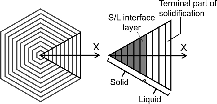
Shape of a cross section perpendicular to the growing direction of a dendrite arm and the analytical region applied for the mathematical model.

On the basis of the above assumptions, a model has been created as follows. Diffusion of the solutes in the solid phase is calculated according to the following equation:   

$$\frac{\partial C_{\gamma }}{\partial t}=\frac{\partial }{\partial x}\left[D(T)\frac{\partial C_{\gamma }}{\partial x}\right]$$(1)

where C_γ is concentration of a solute in the solid phase (γ), t is time, x is distance from the center of a dendrite arm and D(T) is diffusion coefficient as a function of temperature.

The analytical layers in Fig. 1 are divided into 50 elements. Then, microsegregation profiles of the solutes during and after solidification can be calculated by a finite difference method.

At the solid and liquid interface, local equilibrium is maintained at all times as follows:   

$$C_{\gamma }^{*}=k{C}_L$$(2)

where $C_{\gamma }^{*}$ is the solute content in the solid phase (γ) at the interface, k is the partition coefficient and C_L is the solute content in the residual liquid phase. The interface between the solid and liquid phases is allowed to advance by one element along the x-axis. Liquidus temperature of the residual liquid phase is obtained by the following equation at a given time:   

$$T_L=T_M+{\sum }_i^n{m}_i\mathrm{\Delta }{C}_i$$(3)

where T_L is the liquidus temperature of the residual liquid phase, T_M is the liquidus temperature of the initial alloy composition, m_i is the decrement of liquidus temperature per 1 mass% solute i, ΔC_i is increment of concentration from the initial concentration.

2.3. Parameters

Diffusion length of the analytical region was determined as 25.5 μm corresponding to a half value of the average secondary arm spacing of 51 μm. Table 2 shows the partition coefficients¹¹⁾ and m-values obtained by FactSage ver.7.0¹⁴⁾ with the database of FSStel. Equilibrium partition coefficients obtained by the iso-thermal experiments¹¹⁾ were applied for Eq. (2).

Table 2. Partition coefficients and m-values of the solutes.

	Cr	Ni	Mo	Cu
k (–)	0.89	1.02	0.57	0.79
m (K/mass%)	−3.38	−1.10	−5.27	−6.66

Table 3 shows the variation of diffusion coefficient of each solute in the solid phase^15,16,17) as a function of temperature. Two datasets of diffusion coefficients in the alloys were used. The first dataset (1) consists of the coefficients in Fe(γ)-X binary systems. The second dataset (2) consists of the coefficients in Fe–Cr–Ni alloys except for Cu, because diffusion coefficient of Cu in Fe–Cr–Ni alloys has not been reported. As for Cu, therefore, the coefficient same as in the dataset (1) was used in the dataset (2). The diffusion coefficients are plotted as a function of temperature as shown in Fig. 2. It is noted that the lines are those extrapolated to the temperature range from 1573 to 1673 K. As can be seen, the diffusion coefficients of Cr, Ni and Mo in the Fe–Cr–Ni systems are higher than those in the Fe(γ)-X binary systems approximately by one order per digit. It is worthy to note that Mo diffuses the fastest in the both cases. Figure 3 shows the effect of each solute on the liquidus temperature. Calculation started at 1675 K, the liquidus temperature of the original alloy system, and finished at 1573 K.

Table 3. Diffusion coefficients of the solutes in the solid phase.

Dataset	Solutes	D(γ) (cm2/s), D=D0exp[−Q/(RT)]		Alloy	Ref.
		D0 (cm2/s)	Q (cal/mol)
(1)	Cr	0.17	63098	Fe(γ)-X	15
	Ni	0.77	67161
	Mo	0.036	57361
	Cu	0.43	66922
(2)	Cr	0.19	58300	Fe-25Cr-20Ni	16
	Ni	4.06	67500
	Mo	1.68×10−4	34082	SUS316	17
	Cu	0.43	66922	Fe(γ)-X	15

Fig. 2.

Variation of diffusion coefficients of the solutes in the solid phase with temperature.

Fig. 3.

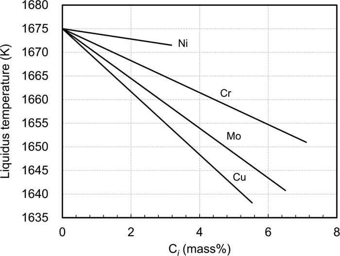
Effect of each element on the decrease in liquidus temperature.

3. Results

3.1. Modeling Results for Variation of Solutes Concentration as Time

Figures 4(a) to 4(d) show the profiles of the elements in the solid and liquid phases of the model calculation applying the condition with the dataset (1) in Table 3. Figures 4(a) to 4(d) show the profiles of (a) before solidification, (b) 2.7 s (c) 18.8 s and (d) 64 s after solidification. The solid fractions of Figs. 4(a) to 4(d) correspond to 0, 0.1, 0.5 and 0.9, respectively. The solute contents start with kC_i at the position of fs=0 as seen in Fig. 4(b). As solidification progresses in Figs. 4(b), 4(c) and 4(d), Cr, Mo and Cu become more concentrated in the liquid phase. Their contents in the solid phase also become higher according to the partition coefficient of each element. Obviously, the solutes of Cr, Mo and Cu are concentrated in the liquid phase at fs=0.9 as can be seen in Fig. 4(d). Meanwhile, Ni shows the behavior opposite to Cr, Mo and Cu due to the k value of 1.02.

Fig. 4.

Profiles of the elements in the solid and liquid phases of (a) before solidification, (b) 2.7 s, (c) 18.8 s and (d) 64 s after solidification.

3.2. Post Solidification Behavior

Figures 5(a) and 5(b) show the profiles of the elements in the solid phase at the moments when (a) solidification is completed and (b) the alloy is subsequently cooled down to 1573 K. Cr, Mo and Cu contents increase in the fs range from 0.9 to 1. Focusing on the difference between Figs. 5(a) and 5(b), Cr and Mo contents significantly decrease during cooling after solidification. On the other hand, Ni shows the behavior opposite to Cr, Mo and Cu. This fact shows that diffusion of the solutes during cooling process cannot be ignored even though it is quite a short period.

Fig. 5.

Profiles of the elements in the solid phase at the moments when (a) solidification is completed and (b) the alloy is subsequently cooled down to 1573 K.

4. Discussion

4.1. Profiles at Solidification Completion

Figure 6 shows the profiles of the solute contents at the moment of solidification completion. This figure indicates the effect of the diffusion datasets (1) and (2) listed in Table 3. The solid and dashed lines show the results using the datasets (1) and (2), respectively. The solid lines are the same as those in Fig. 5(a). The position at fs=0 corresponds to the dendrite arm core, while the position at fs=1 corresponds to the interdendritic region. Cr, Mo and Cu contents increase with increasing fs due to the k values lower than 1. On the other hand, Ni content decreases with increasing fs due to the k value of 1.02. Remarkable difference between the datasets (1) and (2) is obviously seen as for the Cr and Mo lines. It can be seen that the lines with the dataset (2) are lower than those with the dataset (1) in the region of fs above 0.8. In the region of fs below 0.8, contrary, these lines with the dataset (2) are higher than those with the dataset (1). This shows that diffusion coefficient affects the calculation results, so that one should carefully select data.

Fig. 6.

Calculated concentration distributions of the solutes, where two datasets (1) and (2) of the diffusion coefficients listed in Table 3 are applied for the timing of solidification completion.

4.2. Arrangement of the Experimental Data

Figure 7 shows the calculated lines of the solutes at the timing cooling down to 1573 K in comparison with the previous experimental data plots.¹¹⁾ In the previous report, the data were simply arranged in increasing order for Cr, Mo and Cu and in decreasing order for Ni. It has to be noted that the way to arrange in this study is different from the previous way. It is postulated that the law of mass conservation has to be satisfied at each fs point to correctly arrange the data. The summation of all the components of Fe, Cr, Ni, Mo and Cu, have to be 100 mass% at each fs point. Therefore, the data were rearranged as Fe content simply decreased, while Cr, Ni, Mo and Cu contents were rearranged dependently with the Fe content at each fs point. Due to this reason, scattering to some extent can be seen differently from the previous plots.¹¹⁾

Fig. 7.

Calculated concentration distributions of the solutes, where two datasets (1) and (2) of the diffusion coefficients listed in Table 3 are applied for the timing of cooled down to 1573 K, compared with the previous data plots experimentally measured by EDS.

4.3. Profiles after Solidification

It can be seen in Fig. 7 that the dashed lines of Cr and Mo with the dataset (2) pass below the solid lines with the dataset (1) in the fs region above 0.6. This is caused by the higher diffusion coefficients of Cr and Mo in the Fe–Cr–Ni system than in the Fe(γ)-X system. In addition, the dashed lines for Cr and Mo pass below the plots in the high fs region. This tendency after solidification is more enhanced than that at the moment of solidification completion shown in Fig. 6. For Ni and Cu, the calculated lines are mostly consistent with the experimental data.

Firstly, the lines of Cr and Mo show significant difference between the datasets (1) and (2) particularly in the higher fs region. As for Cr, the solid line of the dataset (1) passes above the plots in the region of fs above 0.5, while the line passes below the plots in the region of fs below 0.5. On the other hand, the dashed line of the dataset (2) passes below the plots in the region of fs above 0.8, while the line passes above the plots in the range of 0.2 to 0.8 in fs.

As for Mo, the solid line of the dataset (1) passes above the plots in the region of fs above 0.7, while the line passes below the plots in the region of fs below 0.7. On the other hand, the dashed line of the dataset (2) passes below the plots in the region of fs above 0.7, while the line passes above the plots in the range of 0.2 to 0.7 in fs.

Here, it is quite important to focus on the initial compositions at fs=0 because they would start with the values of kC_i0 in principle. The corresponding values are 25.3, 17.7, 2.6 and 1.2 mass% for Ni, Cr, Mo and Cu, respectively, as pointed in Fig. 7. It is clearly realized that the plots at fs=0 is higher than the values of kC_i0 except for Ni. In addition, the plots of Cr and Mo at fs=0 well agree with the dashed lines. These agreements continue approximately up to 0.2 in fs.

Before the study, we presumed that the dendrite core would not be affected by back diffusion in the experiment. This was because the experiments were carried out with the relatively fast cooling rates. The good agreement of the plots with the dashed line implies that back diffusion during and after solidification affects as deeply as the dendrite core region. In this view, the dashed lines of the dataset (2) are more consistent with the solidification behavior in the relatively low fs region. This result is quite reasonable because the application of the dataset (2) by the Fe–Cr–Ni systems, similar to the present system, would give us more accurate estimations. Whereas, the behavior in the relatively high fs region is really different from that in the low fs region. As explained above, the dashed Mo line of the dataset (2) passes below the plots in the region of fs above 0.7. The same tendency is seen on the dashed Cr line in the region of fs above 0.8.

On the other hand, Ni content decreases with fs due to the partition coefficient of 1.02. Thus, one should pay attention to the position at fs=1. As mentioned above, the two lines are quite close to each other. However, when carefully focusing on the position at fs=1, the dashed line of the dataset (2) consistently passes through the group of the plots. The above results suggest that it is appropriate to apply the diffusion coefficients obtained by the alloy systems similar to the present system.

As for Cu, the line passes below the plots whole through all the fs points. This is probably caused by the accuracy of EDS analysis because the peak of Cu is partially overlapped with that of Ni. Furthermore, the peak of Cu is lower than Ni due to the original composition.

4.4. Problems Associated with Segregation Model

It is required to clarify the reason why the dashed lines do not agree with the plots in the region of relatively high fs. Considering the formation of microsegregation, the most important position is the interdendritic region at fs=1. The possible problems to bring this disagreement are considered as follows:

(a) Diffusion coefficients of Cr and Mo may be lower in the region where Cr and Mo are concentrated.

(b) Diffusion coefficients of Cr and Mo may be lower in the alloy systems containing Cu.

(c) Diffusion coefficients used in this study are those measured below 1573 K.

(d) Partition coefficients may vary with solidification progress.

(e) Solutes in the residual liquid may not be homogeneously distributed but concentrated in front of a dendrite tip.

(f) Two-dimensional concept may not adequately reflect the ratio of solid/liquid interfacial area to solid volume.

The following tasks should be made to create a more accurate model accounting for the above problems. Firstly, diffusion coefficients should be measured in the range of the post solidification temperatures, relevant to the problems (a), (b) and (c). Partition coefficients should be measured as a function of fs relevant to the problem (d). A recent study¹⁸⁾ has shown that the partition coefficients k of Cr, Ni and Mo vary with solidification by the in-situ measurement of SUS316 stainless steel. This is related to the problems (d) and (e).

In addition, according to a recent study,¹⁹⁾ three-dimensional evolution of specific interfacial area was calculated as a function of fs. The specific interfacial area mentioned in the paper¹⁹⁾ means the ratio of solid/liquid interfacial area to solid volume. The result indicated that the specific interfacial area was obtained as a smooth curve taking a maximum value at fs close to 0.5. In the present study, the specific interfacial area simply increases with increasing fs. This fact suggests that the ratio of the interfacial area to the solid volume should be considered three-dimensionally in relation with the problem (f).

4.5. Mechanism of “Slope Segment” in Random Sampling Method

The pioneering work¹³⁾ suggests that the fs range between 0.1 and 0.6 should be taken for the determination of k values.^11,13) The reason to eliminate the data in the region of fs below 0.1 is attributed to the occurrence of the “slope segment”, which is so called “edge drop” toward the position at fs=0. However, the mechanism of the “slope segment” was not described in the paper.¹³⁾ In Fig. 7, the “edge drop” toward fs=0 corresponding to the “slope segment” is not seen.

In the present study, as explained earlier, the data taken by EDS analyses were rearranged as Fe contents simply decreased, while the other elements were dependently associated with Fe contents to keep the law of mass conservation. As a result, some extent of scatters appeared in comparison with the previous smooth plots.¹¹⁾ Therefore, the “slope segment” is most likely resulted from the measurement error originated by EDS analyses. As usually recognized, the measurement involves error to some extent caused by various reasons. It should be emphasized that the slope segment, which seemed somewhat tricky, can be avoided by the present way of arrangement.

On the other hand, the suggestion to eliminate the data in the range of fs above 0.6 is attributed to the concentration of the solute. Due to this fact, the data plots do not show a linear function when taking ln (1-fs) and ln (C_s/C₀) on X and Y-axes, respectively. This implies that partition coefficient may vary with an increase in fs.

As summarized, it is quite expected that experimental approach should be made to clarify the behavior in the region of fs above 0.9. The experimental work should be carried out to solve the problems mentioned above. Firstly, diffusion coefficients applicable for the post solidification temperatures should be measured. Secondly, the effect of fs on the partition coefficients should be clarified. Further, the ratio of the interfacial area to the solid volume should be considered three-dimensionally. Finally, a model based on three-dimensional concept should be developed.

5. Conclusions

Microsegregation of a Fe–Cr–Ni–Mo–Cu alloy was studied using the calculation model on the basis of two-dimensional concept considering diffusion of solutes during and after solidification. Two datasets of diffusion coefficients obtained by the Fe(γ)-X binary and the Fe–Cr–Ni systems were applied for the model in comparison with the previous experimental results. In addition, the experimental data were rearranged as Fe content simply decreased, while Cr, Ni, Mo and Cu contents were rearranged dependently with the Fe data at each fs point to keep the law of mass conservation. The following words summarize this study.

(1) The calculations of Cr and Mo using the dataset of Fe–Cr–Ni systems fitted the experimental data in the low fs region.

(2) The calculated lines of Cr and Mo passed below the experimental data in the high fs region.

(3) The above fact could be attributed to the following problems:

 (a) Diffusion coefficients might be lower at the post solidification temperature.

 (b) Partition coefficients might vary with solidification progress.

 (c) The ratio of the solid/liquid interfacial area to the solid volume might vary with solidification progress.

(4) The following work should be conducted to solve the above problems:

 (a) Diffusion coefficients applicable for the post solidification temperatures should be measured.

 (b) The effect of fs on the partition coefficients should be clarified.

 (c) The ratio of the interfacial area to the solid volume should be considered three-dimensionally.

(5) The present arrangement showed that the “slope segment” appearing in the region of fs below 0.1 in random sampling method was attributed to the probable measurement error of EDS analyses.

References

• 1)   M.  Yabe and  N.  Koide: Tetsu-to-Hagané, 99 (2013), 415.
• 2)   E.  Scheil: Z. Metallkd., 34 (1942), 70.
• 3)   H. D.  Brody and  M. C.  Flemings: Trans. Metall. Soc. AIME, 236 (1966), 615.
• 4)   T. W.  Clyne and  W.  Kurz: Metall. Trans. A, 12 (1981), 965.
• 5)   I.  Ohnaka: Trans. Iron Steel Inst. Jpn., 26 (1986), 1045.
• 6)   T.  Matsumiya,  H.  Kajioka,  S.  Mizoguchi,  Y.  Ueshima and  H.  Esaka: Trans. Iron Steel Inst. Jpn., 24 (1984), 873.
• 7)   Y.  Ueshima,  S.  Mizoguchi,  T.  Matsumiya and  H.  Kajioka: Metall. Trans. B, 17 (1986), 845.
• 8)   C.  Ji,  S.  Luo,  M.  Zhu and  Y.  Sahai: ISIJ Int., 54 (2014), 103.
• 9)   T.  Sawai,  Y.  Ueshima and  S.  Mizoguchi: ISIJ Int., 30 (1990), 520.
• 10)   K.  Saida,  Y.  Nishijima,  K.  Nishimoto,  K.  Kikuchi and  J.  Nakayama: Weld. J., 92 (2013), No. 11, 322s.
• 11)   K.  Yamamoto,  K.  Narikiyo,  N.  Sasaguri,  H.  Miyahara,  K.  Mizuno and  H.  Todoroki: Tetsu-to-Hagané, 103 (2017), 703.
• 12)   M. N.  Gungor: Metall. Trans. A, 20 (1989), 2529.
• 13)   W.  Yang,  K.-M.  Chang,  W.  Chen,  S.  Mannan and  J.  DeBarbadillo: Metall. Mater. Trans. A, 31 (2000), 2569.
• 14)   C. W.  Bale,  E.  Bélisle,  P.  Chartrand,  S. A.  Decterov,  G.  Eriksson,  K.  Hack,  I.-H.  Jung,  Y.-B.  Kang,  J.  Melançon,  A. D.  Pelton,  C.  Robelin and  S.  Petersen: Calphad, 33 (2009), 295.
• 15)  Metals Data Book, ed. by Y. Waseda, The Japan Institute of Metals, Maruzen, Tokyo, (2004), 22.
• 16)  Solidification of Steels, ed. by K. Ohsasa, The 19th Committee on Steelmaking, JSPS, Tokyo, (2009), Appendix, 42.
• 17)  Stainless Steels Handbook, ed. by R. Tanaka, Japan Stainless Steel Association, Tokyo, (1994), 158.
• 18)   I.  Uwabe,  K.  Dobara,  K.  Morishita,  T.  Nagira and  H.  Yasuda: Tetsu-to-Hagané, 103 (2017), 678.
• 19)   H.  Neumann-Heyme,  K.  Eckert and  C.  Beckermann: Acta Mater., 140 (2017), 87.