Abstract
A three-dimensional mathematical model of an industrial Single Snorkel Refining Furnace (SSRF) was implemented in designed experiments to investigate the influence of injection position and snorkel diameter on mixing efficiency and circulation rate. The discrete phase model–volume of fluid coupled model was employed to describe the argon/steel/slag/air multiphase flow. The expansion behavior of argon bubbles was considered. The results indicated that eccentric injection is greatly beneficial for increasing circulation rate and decreasing mixing time. The effect of snorkel diameter was investigated in light of eccentric plug position. It was found that the oversized and undersized snorkel diameter are not desirable, as it contributes poor mixing at ladle bottom and periphery of snorkel, respectively. An optimum diameter was recommended according to a principle that the stirring energy of plume should be distributed reasonably for achieving homogeneous flow in the whole bath.
1. Introduction
Recently, corresponding to the increasing demands for high-purity steel, the vacuum degasser ratio of converter and electric furnace steel has increased rapidly, and various vacuum refining technologies have been developed continually. To satisfy the higher treatment efficiency of refining equipment, the Single Snorkel Refining Furnace (SSRF) has been developed as a revolutionary vacuum refining equipment since the 1970s by Zhang through the reformation of the RH in China.1) Subsequently, a similar vacuum degasser called the Revolutionary Degassing Activator (REDA) was independently exploited by Nippon Steel Corporation in Japan starting in the 1990s, via modification of the DH.2,3,4) Numerous industrial test results proved that the SSRF or REDA shows great superiority in the production of ultra-low carbon steel and ultra-low sulphur steel.5,6,7,8)
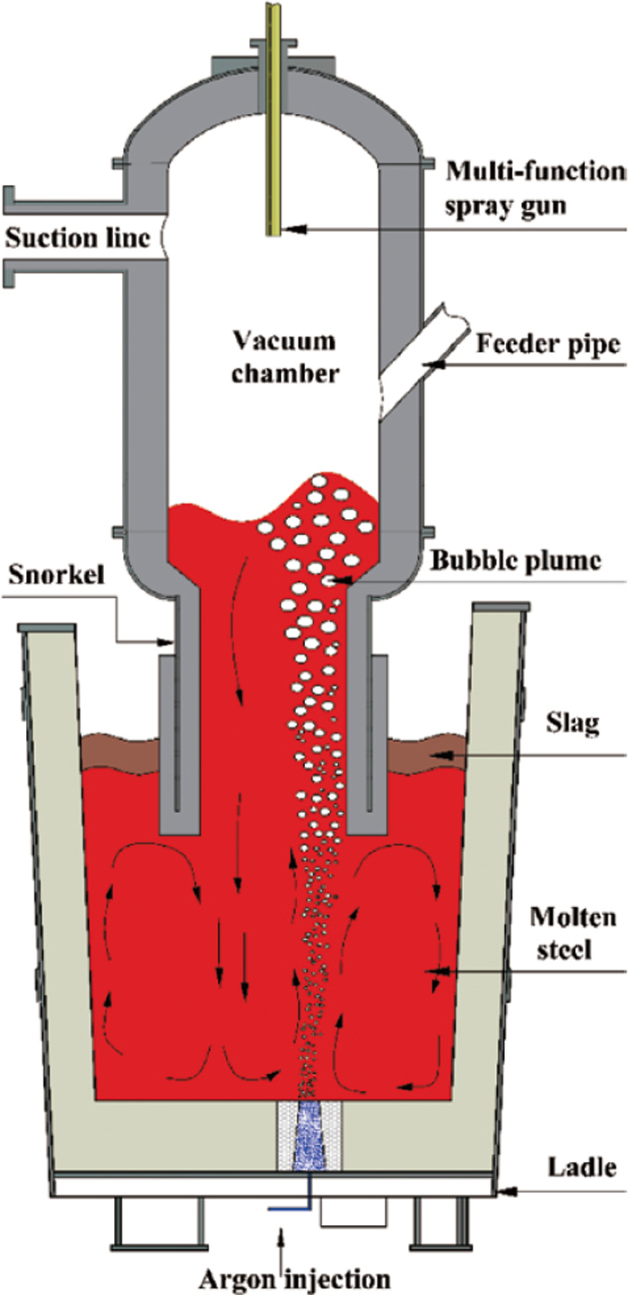
As depicted in Fig. 1, the SSRF consists of ladle, snorkel, vacuum chamber, and feeder bin. During SSRF process, a snorkel is immersed into molten steel, and argon is injected into the ladle through the porous plug at the ladle bottom. Owing to the drive of dispersed argon bubbles, the molten steel is pumped into vacuum chamber via the snorkel, and then continuous circulation is built between ladle and vacuum chamber. Furthermore, various experimental and industrial investigations on SSRF have been performed. The SSRF has been used for degassing, deoxidation, decarburization, desulphurization, adjusting chemical compositions and inclusion removal.9,10,11,12) All of which greatly depend on its flow behavior. Thus, to improve the refining efficiency, it is important to elucidate the mechanism of fluid flow in SSRF process.
Generally, the circulation rate and mixing time are regarded as the prominent indicators that influence the refining efficiency. Kitamura et al.13) conducted industrial mixing tests using the 175 t and 350 t REDA, and the results proved that mixing characteristic of ladle was not deteriorated by the immersion of large snorkel. With the limitation of temperature, the flow field in the actual SSRF has hardly been observed and tested. Therefore, water model and numerical simulation are usually adopted to investigate flow characteristics of industrial SSRF. Aoki et al.14) studied REDA process by developing a cold model to compare the surface decarburization rate with RH, DH, and Tank. Qin et al. and Rui et al.15,16) developed a physical model to investigate the effect of various design parameters on flow field and mixing phenomena, such as injection position, snorkel diameter, and submerged depth.
Recently, two mathematical models have been widely applied to simulate metallurgical flow: the Eulerian–Eulerian method and the Eulerian–Lagrangian method. Detailed comparisons between the two models have been reported.17,18,19,20) Several numerical studies have been performed to investigate the flow field using the Eulerian–Eulerian model in SSRF process.21,22,23) In these studies, the free surfaces of molten steel in ladle and vacuum chamber were usually assumed to be flat and frictionless, and bubble expansion and slag layer were ignored. As observed in ladle experiment,24) the agitation gas injected by the porous plug is dispersed into discrete bubbles. Thus, it is inadequate to deal with discrete bubbles using the Eulerian method. The discrete phase model (DPM), which provides a valid approach to describe the motion of dispersed bubbles, has been widely utilized in some types of industrial reactors, such as gas-stirred ladle,25,26,27,28,29) RH,30,31) and BOF.32,33) In these studies, a coupled mathematical model was mostly employed to track interfacial behaviours using the VOF model and describe bubble motion with the DPM model. The results showed that the calculated value could be well-validated with experimental data from water model. Moreover, the influence of bubble expansion should not be ignored, especially in vacuum refining. Cao et al.29) found that the mixing time is shortened with consideration of bubble expansion in a gas-stirred ladle. Chen et al.31) reported a significant increase in circulation rate when the expansion was considered in an industrial RH reactor. However, the impact of expansion was rarely considered in reported simulations involving SSRF. It is worth noting that a higher expansion ratio of agitation gas is obtained in SSRF because of the greater injection depth compared with RH reactor. Thus, it is necessary to consider the expansion of gas in numerical model for making simulation as realistic as possible.
In the present study, a transient mathematical model was established to simulate multiphase flow in an industrial SSRF. The VOF model in Eulerian frame was employed to track interfaces among the slag/steel/air phases in ladle and vacuum chamber. The DPM was used to solve trajectories of dispersed argon bubbles, and the volume expansion of discrete bubbles was considered on the basis of the ideal gas law. The simulated results for mixing time and local velocity of water were verified via experimental measurements in a 1/3 scale air-water model. The main objective of the investigation was to assess the influence of injection position and snorkel diameter on flow field and mixing efficiency and to supply the further advices to industries.
2. Mathematical Model
In the present work, the multiphase flow in the SSRF reactor has been simulated using the Eulerian-Lagrangian approach based on the following assumptions:
(a) The continuous phases are defined as Newtonian, viscous and incompressible.
(b) The heat transfer between the phases is neglected.
(c) Spherical-shaped bubbles are injected from the ladle bottom, the deformation of the gas bubbles is not taken into account, and the coalescence, collision and breakup of bubbles are ignored.
(d) The injected bubbles generate an additional turbulent kinetic energy on continuous phases, However, obtaining the bubble-induced turbulence is still an unsolved problem because the fraction of the induced energy converted into the steel has a different description and it varies with the researchers.34,35,36) Further improvements are required to consider the effect of bubble induced turbulence and increased viscous dissipation.
(e) All of slag phase is placed into the ladle, there is no top slag in the vacuum chamber.
2.1. VOF Model
The VOF model is employed in this work for tracking the free surfaces among the steel, slag, and air. The tracking is accomplished via the solution of a continuity equation for the volume fraction. For the i-th phase, the continuity equation is described as:
|
1
ρ
i
[
∂
∂t
(
α
i
ρ
i
)+∇⋅(
α
i
ρ
i
u
m
)
]=0
| (1) |
where
ρi is density of gas phase (
i=
g), slag phase ((
i=
s) and steel phase ((
i=
l),
um is mixture velocity, and the volume fraction
αi is solved according to the following constraint:
A single momentum equation is solved throughout the computational domain, and the resulting velocity field is shared among phases. The momentum equation is expressed as:
|
∂
∂t
(
ρ
m
u
m
)+∇⋅(
ρ
m
u
m
u
m
)=
-∇P+∇⋅[
μ
m
(∇
u
m
+∇
u
m
T
)
]+
ρ
m
g+
F
b
| (3) |
|
ρ
m
=
α
l
ρ
l
+
α
s
ρ
s
+
α
g
ρ
g
| (4) |
|
μ
m
=
α
l
μ
l
+
α
s
μ
s
+
α
g
μ
g
| (5) |
where
ρm and
μm are mixture density and viscosity,
P is the pressure, and
Fb represents the force of bubbles acting on liquid phases.
2.2. Discrete Phase Model
Argon bubbles are treated as the discrete second phase. The trajectories of the bubbles are calculated in time and space according to Newton’s Second Law, which is written in the Lagrangian reference frame, given as:
|
d
u
b
dt
=
F
G
+
F
B
+
F
VM
+
F
D
| (6) |
where the left-hand side represents the acceleration of each bubble, and
ub is the velocity of an individual bubble. The forces acting on the bubble are given on the right-hand side of the equation, including the gravitational force, buoyancy force, virtual mass force and drag force. The formulas of the forces are described as follows.
The drag force is viscous resistance of the steel acting on the bubbles and can be expressed as follows:
|
F
D
=
3
μ
m
C
D
R
e
b
4
ρ
b
d
b
2
(
u
m
-
u
b
)
| (7) |
where
ρb is the density of the bubble,
db is the diameter of bubble,
Reb is a function of the relative Reynolds number, and
CD is the drag coefficient. Their expressions are described as:
|
R
e
b
=
ρ
m
d
b
|
u
m
-
u
b
|
μ
m
| (8) |
|
C
D
=
a
1
+
a
2
R
e
b
+
a
3
R
e
b
2
| (9) |
where
a1,
a2, and
a3 are constants suitable for spherical bubble over several ranges of the Reynolds number given by Morsi and Alexander.
37)
The combined action of the gravitational force and buoyancy force on bubble is given as
|
F
G
+
F
B
=
(
ρ
b
-
ρ
m
)
ρ
b
g
| (10) |
As a bubble accelerates across the steel, the surrounding liquid is carried with the same acceleration as the bubble. Therefore, the extra force due to the resistance of the liquid mass is called the virtual mass force and defined as:
|
F
VM
=
C
VM
ρ
m
ρ
b
d
dt
(
u
m
-
u
b
)
| (11) |
where
CVM is the virtual mass coefficient, which represents the volume ratio of the liquid added to the bubble and is set as 0.5 for spherical bubble.
The two-way coupling model is implemented to facilitate momentum exchange between the discrete phase and continuous phase. A momentum source is added to the continuous phase momentum by summing the local contributions from each bubble in the continuous phase flow field.
|
F
b
=
-
∑
i
N
b,cell
(
3
μ
m
C
D,i
R
e
b,i
4
ρ
b,i
d
b,i
2
(
u
m
-
u
b,i
)+
C
VM
ρ
m
ρ
b,i
d
dt
(
u
m
-
u
b,i
)
)
ρ
b,i
Q
b,i
Δt
| (12) |
where
Nb,cell number of bubbles in a particular cell,
ρb,iQb,i is the mass flow rate of argon as bubble and Δ
t is the time step.
The standard two-equation k−ε model is used to describe turbulence. The equations for the turbulence kinetic energy (k) and the turbulent dissipation rate (ε) are written as:
|
∂
∂t
(k
ρ
m
)+∇⋅(
ρ
m
k
u
m
)=∇[
(
μ
m
+
μ
t
σ
k
)
∇k
]+
G
k
-
ρ
m
ε
| (13) |
|
∂
∂t
(ε
ρ
m
)+∇⋅(ρε
u
m
)=∇[
(
μ
m
+
μ
t
σ
ε
)
∇ε
]
+
ε
k
(
C
1ε
G
k
-
C
2ε
ρ
m
ε)
| (14) |
|
μ
t
=
ρ
m
C
μ
k
2
/ε
| (15) |
Where μt is the turbulent viscosity, Gk is the generation of turbulence kinetic energy due to the mean velocity gradients. C1ε, C2ε, Cμ, σk and σε are the empirical constants with values of 1.44, 1.92, 0.09, 1.0 and 1.3, respectively.
2.3. Bubble Size Model
The expansion of bubbles is considered in the current model. Iguchi et al.38,39) reported that heat transfer between cold bubbles and hot liquid is almost completed near the exit of the plug. In order to ensure argon volume flux is equal between the present model and actual condition, the volume of injected argon is amended at standard condition because the heat transfer equation is not considered in the present model, which is calculated as follows:
|
Q
in
=
Q
0
⋅
T
l
T
0
| (16) |
Here, Qin is the flow rate of argon injection in the present model (L/min), Q0 is the is the flow rate of argon injection at actual process (NL/min). Tl, T0 are the temperatures of liquid in actual process and standard condition, 1873 K and 273.15 K, respectively.
In the DPM program, the amount of injection argon is input in the form of mass flow rate (kg/s), which is calculated as follows:
|
m
b
=
Q
in
⋅
ρ
Ar
⋅1.67×
10
-5
| (17) |
Where ρAr is density of bubble at 101325 Pa and 1873 K (kg/m3).
When bubbles are injected from the ladle bottom, the initial diameter of bubbles is calculated by the following expression based on the experimental formula;40,41)
|
d
b,0
=0.091
(
σ
ρ
l
)
0.5
u
b,0
0.44
| (18) |
where
ub,0 is injection velocity of bubble at the exit of plug (m/s), calculated as:
29)
|
u
b,0
=
Q
0
A
⋅1.67×
10
-5
| (19) |
where
A is the cross-sectional area of plug (m
2).
During the process of bubble rising, the density (ρb,t) and diameter (db,t) are calculated at each time step according to the local static pressure:
|
ρ
b,t
=
ρ
b,0
P
V
+
ρ
l
g(H-z)
P
V
+
ρ
l
gH
| (21) |
|
ρ
b,0
=
ρ
Ar
P
V
+
ρ
l
gH
P
0
| (20) |
|
d
b,t
=
d
b,0
(
ρ
b,0
ρ
b,t
)
1/3
| (22) |
Where P0 is the standard pressure (101325 Pa), PV is the pressure in vacuum chamber (Pa), H is the liquid height along the vertical direction from ladle bottom to the free surface in vacuum chamber (m), z is the coordinate position of gas bubble in the vertical direction (m), ρb,0 is the initial bubble density at ladle bottom (kg/m3). The calculated ρb,t and diameter db,t are returned to solve force equations containing Eqs. (7), (10), and (11).
2.4. Definition of Circulation Rate and Mixing Time
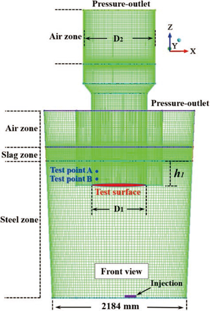
The circulation rate of SSRF is defined as the mass exchanging rate of steel between ladle and vacuum chamber. As shown in Fig. 2, the cross section at the exit of snorkel is selected as test surface to calculate the circulation rate. Since the upflow and downflow coexist in the snorkel, the test surface is divided into two parts according to the positive and negative of vertical velocity of steel, representing the area occupied by the upflow and downflow respectively. The mass flow rate through the area is computed as follows;
|
M=
∑
i=1
n
ρ
l
⋅
u
i
z
⋅
A
i
| (23) |
Where n is the mesh number at the surface, Ai is projected area of cell at the surface,
u
i
z
is the vertical velocity of steel. Actually, if a quasi-steady state is reached, the mass flow rate of upflow and downflow are almost equal. The circulation rate of SSRF is defined as follows:
|
M
cir
=
|
M
up
|+|
M
down
|
2
| (24) |
Where Mcir is circulation rate of SSRF (kg/s), Mup and Mdown are the mass flow rate of upflow and downflow respectively.
The mixing time is calculated by solving species transport equation:
|
∂
∂t
(
ρ
m
C)+∇⋅(
u
m
ρ
m
C)=∇⋅[
μ
m
+
μ
t
Sc
(
∂C
∂
x
i
)
]
| (25) |
Where C is the tracer concentration, and Sc is the turbulent Schmidt number which is set to 0.7. The 95% mixing time is quantified as the all monitoring values within ±5 percent of final concentration (C∞).
3. Boundary Conditions and Solution Procedure
The geometrical parameters and material properties of the 70t-SSRF used in the present study are listed in Table 1. As shown in Fig. 2, the computation domain is divided into four zones depending on the different fluid distribution. The local grid refinement is employed at the interfaces and the bubble plume region. In order to capture the steep gradients with reasonable accuracy on a coarse grid, the no-slip conditions are used at the walls of the ladle, snorkel, and vacuum chamber. The bubbles are allowed to reflect at the above walls. The pressure-outlet boundary condition is adopted on the top surfaces of the vacuum chamber and ladle.
Table 1. Dimensions and material properties of the 70-ton SSRF.
| Parameters | Values |
|---|
| Diameter of ladle (up/down) | 2.450/2.184 m |
| Height of ladle | 3.06 m |
| Weight of slag/molten steel | 2.3/70 ton |
| Diameter of plug | 0.10 m |
| Argon flow rate, Q0 | 100 NL/min |
| Inner diameter of snorkel, D1 | 0.6–1.2 m |
| Inner diameter of vacuum chamber, D2 | 1.3 D1 |
| Length of snorkel | 1.6 m |
| Thickness of snorkel refractory | 0.25 m |
| Pressure of vacuum chamber | 2000 Pa |
| Immersion depth of snorkel, h1 | 0.4 m |
| Interfacial tension of steel-air | 1.823 N/m |
| Interfacial tension of steel-slag | 1.15 N/m |
| Interfacial tension of slag-air | 0.58 N/m |
| Density of molten steel/slag/air | 7020/3500/0.5 kg/m3 |
| Density of discrete phase (argon) at standard pressure and temperature. | 1.785 kg/m3 |
| Viscosity of steel/slag/air | 0.0055/0.05/8.9 × 10−5, Pa·s |
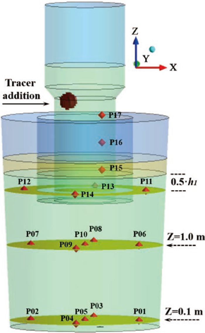
Initially, four zones are filled with the corresponding fluid, and then the bubbles are injected from the plug. The bubbles disappear after arriving at the interface where the volume fraction of air is larger than 0.5 by the function of user-defined. After initialization, the transient simulation is run until a quasi-steady is reached. The criterion of quasi-steady is defined when two conditions are reached: (i) on the test surface, the net mass flow rate of molten steel approaches to zero; (ii) the flow velocity of molten steel reaches stability. Then, the circulation rate is measured based on the Eq. (24), and the tracer is added. The concentration of tracer is detected at seventeen monitoring points as depicted in Fig. 3. Several investigations have clarified that the measurement of mixing time is affected by the monitoring position.42,43) Therefore, it is vital to employ monitoring points as much as possible with the purpose of detailed analysis of the mixing behavior. The CFD-Fluent® 17.0 is employed with user-defined functions to solve the multiphase flow and bubble properties in the SSRF, and the pressure–velocity coupling scheme is employed via the PISO algorithm.
4. Results and Discussion
4.1. Model Validation
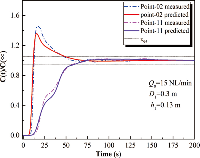
A 1/3-geometric scale air-water model was established to validate the mathematical model. The dimensions and operative parameters of the water model were designed using the similarity criteria based on the modified Froude Number.44) The slag layer was ignored in this section for the water model and mathematical model. The pressure of vacuum chamber was set to 96600 Pa for simulation, which can guarantee liquid (water) level difference of 0.48 m, corresponds to a liquid (steel) level difference of 1.44 m (2000 Pa). The 95% mixing time was measured via a conductivity-measurement technique. A 65-mL saturated KCl solution was injected into the water from the vacuum chamber, and then tracer concentration was detected simultaneously at P02 and P11 as depicted in Fig. 3. Figure 4 shows the results of the measured and predicted tracer concentration as a function of time. It is obvious that the response time and change tendency of the predicted concentration are close to the measured values.
Furthermore, the velocity of the water was measured using a digital differential manometer, which is a simpler version of a Pitot tube. A detailed description of the theory for the velocity measurement is presented in Ref. 43. As shown in Fig. 2, local test point-A and B were selected as the measuring position, where the direction of water velocity is almost vertical. The data were continuously measured for 100 second with a sampling interval of 1 second, and then the average value was taken as the result. Table 2 shows the quantitative comparison between the calculated and measured velocity, it is observed that calculated values reasonably agree well with the measured values. Therefore, the present model provides reliable prediction of both the mixing and local velocity.
Table 2. The comparison of measured velocities with predicted values in the water model.
| Gas flowrate | 10 NL/min | 20 NL/min |
|---|
| Test point | A | B | A | B |
|---|
| Measured (m/s) | 0.181 | 0.176 | 0.245 | 0.238 |
| Calculated (m/s) | 0.184 | 0.182 | 0.257 | 0.248 |
| Relative error (%) | 1.6 | 3.4 | 4.8 | 4.2 |
The gas injection position is a significant design parameter for achieving high-efficiency stirring in the SSRF process. Therefore, the effect of the injecting position on flow field is investigated. As depicted in Fig. 5, four different injecting positions are employed with a linear interval of 0.25 R. (R is the radius of snorkel, m) In these cases, the snorkel diameter is maintained constant (D1 = 0.9 m). and the other parameters are also kept constant as mentioned in Table 1.
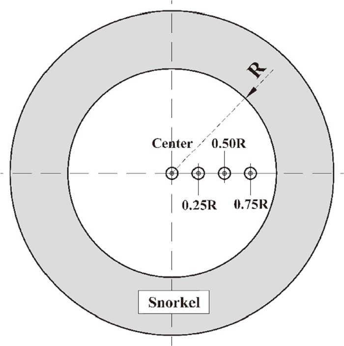
Figure 6 shows the area distribution of the upflow and downflow on the test surface for different injection positions, the calculated circulation rate is given in Table 3 according to area distribution. It can be found that the mass flow rate of the upflow and downflow is nearly equal because of mass conservation. Figure 7(b) illustrates the effect of injection position on the 95% mixing time and circulation rate. Clearly, the mixing time initially decreases then increases as the injection position away from center. The mixing time is minimized at 0.5 R, then increases slightly as the plug position exceeds 0.5 R. However, the circulation rate initially increases, then decreases with the plug position more than 0.25 R.
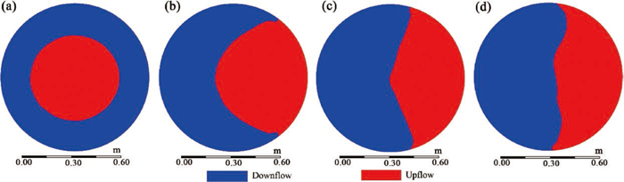
Table 3. The predicted circulation rate for different injection positions.
| Mass flow rate | Gas injection position |
|---|
| Center | 0.25 R | 0.50 R | 0.75 R |
|---|
| Upflow, kg/s | 679.7 | 783.4 | 760.6 | 553.6 |
| Downflow, kg/s | −680.2 | −787.2 | −765.7 | −557.6 |
| Relative error, % | 0.07 | 0.49 | 0.67 | 0.72 |
| Circulation rate, kg/s | 680.0 | 785.3 | 763.2 | 555.6 |
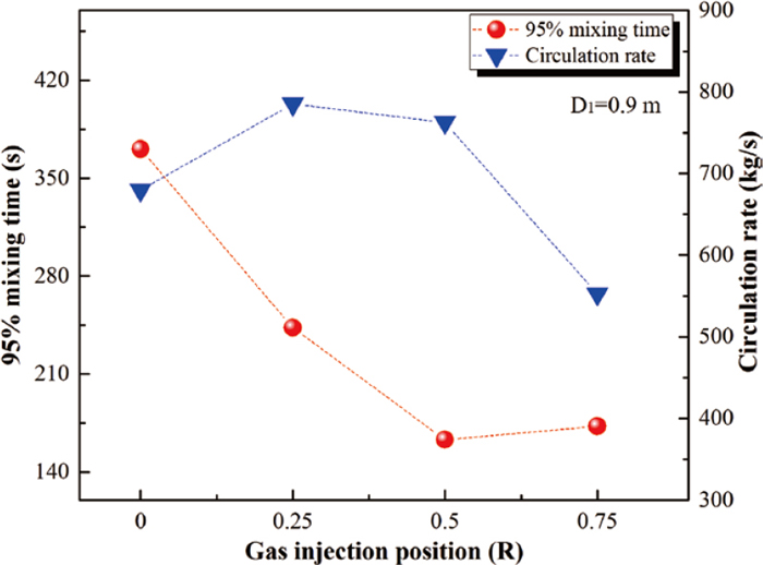
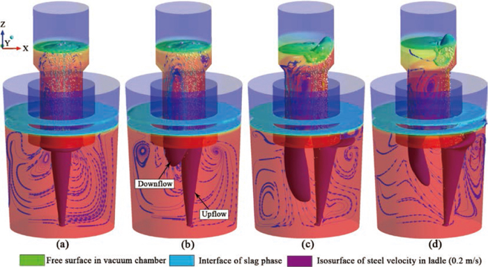
Figure 8 shows the distributions of steel streamlines at the XZ section and the contours of velocity (0.2 m/s) in ladle. It is clear that a recirculation flow, characterized by an upflow and a downflow, is generated between ladle and vacuum chamber. For the case of central injecting, the axisymmetric streamlines are presented in the snorkel, and an annular downflow is formed along the inner wall of snorkel. Actually, this flow distribution easily leads to an increase in contact area between upflow and downflow in the snorkel, and contact area between downflow and snorkel wall is also increased, which means more kinetic energy of downflow is consumed because of increasing viscous dissipation. After the injection position derivates from the center, the downflow is discharged directly from the left side of snorkel with the higher speed than that of central injection. Especially at 0.5 R position, the downflow can even reach the bottom of the ladle. As a result, the stirring efficiency of bottom liquid is enhanced. However, in the case of 0.75 R, it is found that the most of upflow cannot be pumped into the snorkel, so circulation rate is reduced. Besides, because of the great energy of plume, the flow near the snorkel bottom has an increasing tendency to erode the refractory. Consequently, it is concluded that 0.5 R injecting position is beneficial to obtain the higher mixing efficiency and circulation rate.
The inner diameter of the snorkel significantly influences the circulation rate during the SSRF process. In this section, the effect of different diameters, ranging from 0.6 to 1.2 m with 0.1 m increment, is investigated on the basis of the 0.5 R gas injection position. The other parameters are kept constant as mentioned in Table 1. Figure 9 describes the circulation rate with diameters. It can be found that the circulation rate increases as the diameter increases, but after a certain diameter (1.1 m), the circulation rate becomes saturated. Actually, with the increase of the snorkel diameter, the horizontal distance between the plug and the inner wall of the snorkel increases, thus there is an increasing amount of the bubble plume entering the snorkel, and then the circulation rate increases. When the diameter exceeds 1.1 m, all of the bubble plume has completely entered the snorkel. Thus, the circulation rate remains constant.
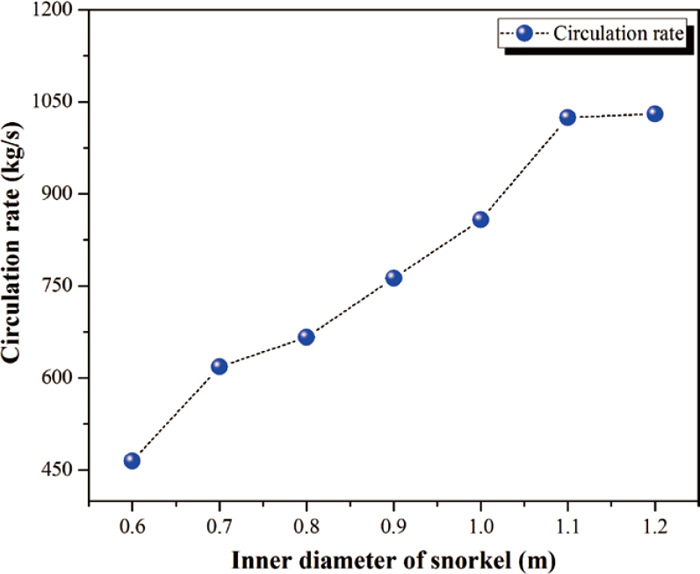
Figure 10 shows the response curves of dimensionless tracer concentration with time as diameter is less than 0.9 m. It is clear that the 95% mixing time continually decreases when the diameter increases from 0.6 to 0.8 m. Furthermore, it is found the tracer concentration monitored at P02 are always the last to reach the 95% mixing time. Thus, it seems that an obvious dead zone exists near P02, which is located at the bottom corner of the ladle. This result can be explained by the fact that small snorkel diameter contributes low circulation rate, and in turn, a weak downflow is generated. It is difficult for the weak downflow impinging into the ladle bottom. Therefore, the steel at the bottom is not easily mixed.

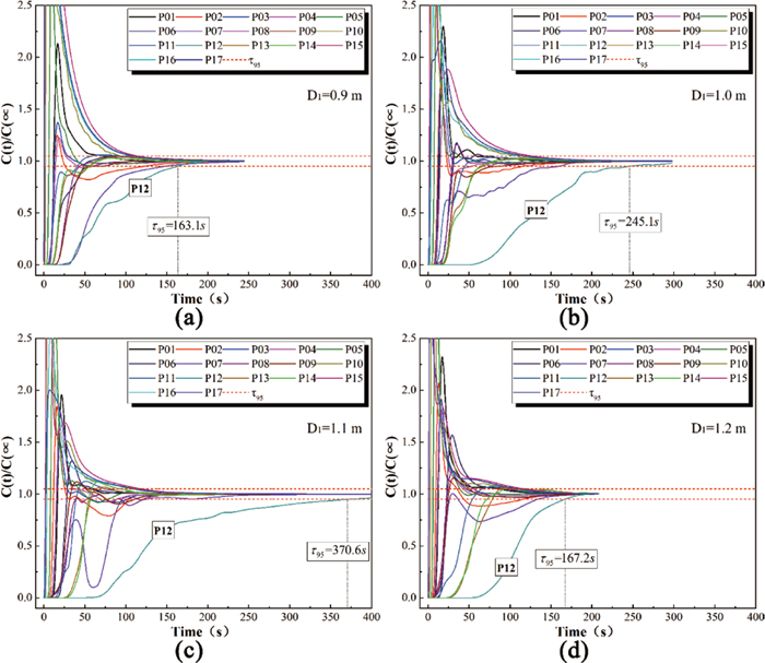
Figure 11 shows the tracer response curves with time as diameter exceeds 0.8 m. It can be seen that the mixing time dramatically increases from 163.1 to 370.6 s with the diameter increasing from 0.9 to 1.1 m. Furthermore, it is obvious that the 95% mixing time is dominated by the local mixing speed of P12. This tendency can be explained by the fact that the increasing diameter results in a reducing amount of bubble plume flowing out of snorkel. Therefore, the mixing speed of the steel around the snorkel is weakened. When the diameter is increased from 1.1 m to 1.2 m, the 95% mixing time steeply declines from 370.6 s to 167.3 s, it seems that the local mixing time of P12 is dramatically shorten. The difference of the mixing time at P12 is discussed later by the comparison of flow fields.
4.3.2. The Analysis of Flow Field
Figure 12 shows the distribution of steel streamlines and contours of velocity (0.2 m/s) for different diameters. It is observed that the steel in ladle is pumped into snorkel along the left side of snorkel, then rises until the upflow reaches the free surface, and then flows into the ladle along the right side of snorkel at a high velocity. With the increase of diameter, it can be seen that the intensified downflow impinges toward the ladle bottom, and then two large recirculation zones are generated along the bottom-side corner. After this process, the steel flows into the snorkel again, the next circulation begins. It is clear from contours of velocity that the impacting depth of downflow increases as the diameter increases, which leads to the disappearance of the bottom dead zone. To quantitatively investigate effect of the diameter on flow field, four horizontal lines are specified at the XZ cross section as depicted in Fig. 13.
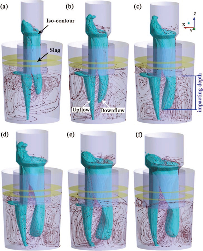
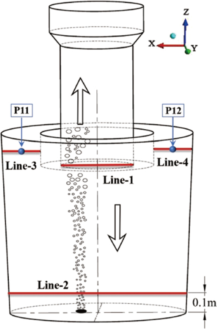
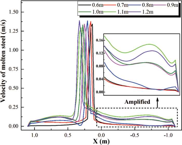
Figure 14 shows the comparison of steel vertical velocity for different diameters, which corresponds to the vertical velocity along the horizontal line-1 at the height of snorkel exit. It is observed that the peak value of upflow velocity slightly increases as diameter increases, but the tendency is not obvious as diameter exceeds 1.1 m, where circulation rate becomes saturated. For the diameters of 0.6 m and 0.7 m, the velocity of upflow near the center of snorkel is higher than other diameters, which means that the average velocity of the upflow is higher than others. Therefore, the velocity of returned downflow is higher. However, with a higher velocity of downflow, it causes a lower impacting depth in ladle. This behavior indicates that the effect of circulation rate on impacting depth is more significant than downflow velocity. For the diameter of 1.2 m, the downflow velocity is lower than that of other diameters. This is because the circulation rate has become saturated as diameter increases to 1.1 m, so the further increased diameter means the increasing of cross section area of snorkel, then velocity is declined.

Figure 15 shows velocity distribution of the steel on the Line-2, which is 0.1 m above the ladle bottom. The steel velocity at ladle bottom increases as diameter increases from 0.8 m to 1.1 m, then slightly decreases at 1.2 m. As the diameter is less than 0.9 m, it is clear that the velocity of the bottom liquid is always lower than others. These results indicate that the circulation rate play a significant role in promoting agitation and mixing at the ladle bottom. Besides, these results also provide a reasonable explanation that the mixing speed of whole steel bath is dominated by bottom P02 as the diameter is less than 0.9 m, because circulation rate is lower, and it is very difficult to make the weak downflow to impinge toward the ladle bottom.
Furthermore, it can be found from the streamlines in Fig. 12 that a part of upflow flows out of the snorkel, then flows into the top left corner, next flows into the top right corner along the snorkel wall. It seems that this part of upflow is acted as the stirring power for the flow around the snorkel. When the diameter increases from 0.6 m to 1.0 m, this stirring power is gradually weakening, then disappears in 1.1 m. Meanwhile, the stirring power is replaced by the upward stream derived from the downflow, as shown in Fig. 16.
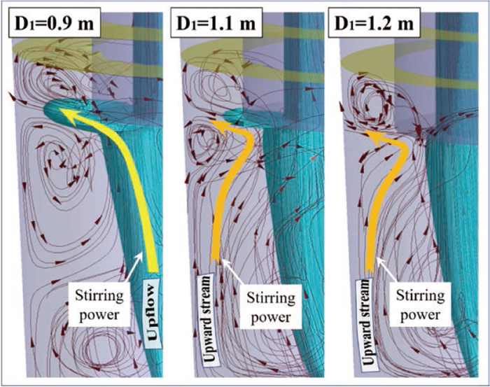
Figure 17 shows the turbulence kinetic energy distribution of the steel on Line-3 and Line-4. Because the stirring power is located in the top left corner, therefore regardless of how the diameter changes, the kinetic energy of the steel on Line-3 is always far larger than that of Line-4. Furthermore, the kinetic energy is severely reduced on both lines as the diameter exceeds 1.0 m. it implies that the replacement of stirring power leads to the poor flowability around the snorkel.
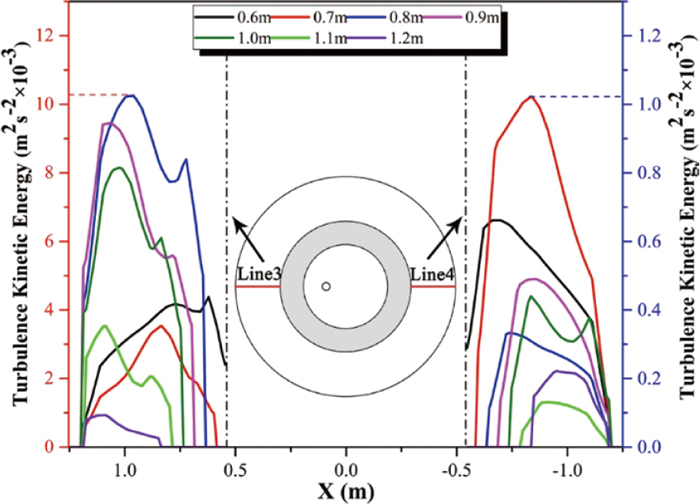
Moreover, in the case of 1.1 m, it is observed that the higher kinetic energy on Line-3 contributes the lower kinetic energy on Line-4 compared with 1.2 m diameter. This phenomenon can be explained by the comparison of the local flow patterns between 1.1 m and 1.2 m. As depicted in Fig. 18. It is clear that there are two horizontal streams around the snorkel, they collide with each other near the P12, the collision causes the poor flow near the P12. After that, they are sucked into the ladle interior along with downflow. Furthermore, at the right corner of ladle bottom, the flow field is characterized by a local recirculation eddy. Because of the higher downflow velocity, the larger eddy height (h′) is obtained in the case of 1.1 m. It means that the sucked stream is blocked by high eddy, therefore the flowability near the P12 is further deteriorated. However, the eddy height (h′) is low in the case of 1.2 m, so the molten steel near the P12 is sucked easily by downflow. Thus, the flowability near the P12 is improved. Besides, this result also provides a reasonable explanation for the abnormal mixing behavior at the P12, as presented in Figs. 11(c) and 11(d).

The effects of the snorkel diameter on the mixing time, circulation rate, and flow pattern are summarized as follows. The undersized diameter is not ideal owing to the poor mixing at ladle bottom and low circulation rate. The larger diameter contributes higher circulation rate, but the problem accompanied as it contributes poor flowability around the snorkel. As a result, there is an increasing possibility of skull at snorkel refractory. All things considered, the diameter of 0.9 m is recommended as the optimum size owing to the shortest mixing time and the homogeneous flow field in ladle.
5. Conclusions
In this study, the VOF-DPM coupled mathematical model was employed to describe the multiphase flow in an industrial SSRF. The effect mechanism of gas injection position and snorkel diameter on the mixing time, circulation rate, and flow field were investigated. The following conclusions are drawn:
(1) The numerical results for the local liquid velocity and mixing time agree well with the experimental measurements. Hence, the multiphase flow in an industrial SSRF can be reliably predicted using the present model.
(2) The injection position of gas strongly influences the flow field in SSRF. The eccentric layout of the injection position is beneficial for improving the mixing efficiency and circulation rate. The optimum eccentric position is 0.5 R under the present conditions.
(3) Increasing the snorkel diameter effectively enhances the circulation rate, but the tendency is not obvious beyond a certain value. Additionally, the oversized diameter is not desirable, as it causes poor stirring around the snorkel. The 0.9 m is recommended as the optimum snorkel diameter in the present study.
(4) To meet the desirable flow field in SSRF, it is important to properly balance the stirring energy distribution of plume between inside and outside of snorkel.
Although the optimum parameters of injection position and diameter were proposed based on the present ladle scale, it is uncertain whether these parameters are suitable for other ladle scales. Further studies should be carried out to investigate effect of ladle scale, such as the ladle capacity is more than 150 t or less than 50 t. Nevertheless, the clarified effect mechanism of these parameters still can provide some references for SSRF design.
Acknowledgement
This work is supported by the National Natural Science Foundation of China (Grant No. 51674024). Thanks very much for the support of the Zhongxing Energy Equipment Co., LTD.
List of symbols
u: Vector velocity (m/s)
P: Pressure (Pa)
Fb: Force of bubbles acting on liquid phases (m/s2)
g: Gravitational acceleration (m/s2)
FG: Gravity (m/s2)
FB: Buoyancy force (m/s2)
FVM: Virtual mass force (m/s2)
FD: Drag force (m/s2)
d: Bubble diameter (m)
CD: Drag coefficient
Re: Reynolds number
Sc: Turbulent Schmidt number
k: Turbulence kinetic energy (m2/s2)
Δt: Time step (s)
C: Tracer concentration
C∞: Tracer concentration of complete mixing state
Q: Gas flow rate (NL/min or L/min)
mb: Mass flow rate of injection argon (kg/s)
M: Mass flow rate of steel (kg/s)
D1: Inner diameter of snorkel (m)
D2: Inner diameter of vacuum chamber (m)
h1: Immersion depth of snorkel (m)
h′: The height of recirculation eddy (m)
Greek Letters
ρ: Density (kg/m3)
α: Volume fraction
μ: Viscosity (Pa·s)
ε: Turbulent dissipation rate (m2/s3)
σ: Interfacial tension (N/m)
Subscripts
m: Mixture phase
l: Steel phase
s: Slag phase
g: Gas phase
b: Discrete argon bubble
b,0: Initial moment of bubbles
References
- 1) J. Zhang: Dalian Special Steel, 3 (1978), 5 (in Chinese).
- 2) K. Miyamoto, H. Aoki and S. Kitamura: CAMP-ISIJ, 11 (1998), 756 (in Japanese).
- 3) H. Aoki, H. Furuta, N. Hirashima and S. Kitamura: CAMP-ISIJ, 11 (1998), 757 (in Japanese).
- 4) H. Aoki, H. Furuta, K. Fujiwara, K. Yamashita, K. Yonezawa and S. Kitamura: CAMP-ISIJ, 11 (1998), 758 (in Japanese).
- 5) H. Sugano, A. Shinkai, K. Kato, K. Miyamoto, K. Yamashita and S. Kitamura: CAMP-ISIJ, 12 (1999), 747 (in Japanese).
- 6) K. Miyamoto, H. Sugano, A. Shinkai, K. Kato, S. Kitamura and K. Yamashita: CAMP-ISIJ, 12 (1999), 748 (in Japanese).
- 7) M. Okimori: Nippon Steel Tech. Rep., 84 (2001), 53.
- 8) Q. X. Rui and G. G. Cheng: Adv. Mater. Res., 476 (2012), 340.
- 9) G. G. Cheng, J. Zhang, N. Z. Yang and F. S. Tong: Special Steel, 15 (1994), 22 (in Chinese).
- 10) J. Zhang, G. G. Cheng, N. Z. Yang and F. S. Tong: Iron Steel, 30 (1995), 19 (in Chinese).
- 11) J. P. Duan, Y. L. Zhang, X. M. Yang, G. G. Cheng and J. Zhang: Steelmaking, 17 (2011), 44 (in Chinese).
- 12) J. P. Duan, Y. L. Zhang, X. M. Yang, G. G. Cheng and J. Zhang: Special Steel, 33 (2012), 26 (in Chinese).
- 13) S. Kitamura, H. Aoki, K. Miyamoto, H. Furuta, K. Yamashita and K. Yonezawa: ISIJ Int., 40 (2000), 455.
- 14) H. Aoki, S. Kitamura and K. Miyamoto: Iron Steelmaker, 26 (1999), 17.
- 15) Z. Qin, M. T. Zhu, G. G. Cheng and J. Zhang: Special Steel, 31 (2010), 5 (in Chinese).
- 16) Q. X. Rui, F. Jiang, Z. Ma, Z. M. You, G. G. Cheng and J. Zhang: Steel Res. Int., 84 (2013), 192.
- 17) J. F. Domgin, P. Gardin and M. Brunet: Proc. 2nd Int. Conf. on CFD in the Minerals and Process Industries, CSIRO, Canberra, (1999), 181.
- 18) D. Guo, L. Gu and G. A. Irons: Appl. Math. Model., 26 (2002), 263.
- 19) M. Madan, D. Satish and D. Mazumdar: ISIJ Int., 45 (2005), 677.
- 20) D. Mazumdar, R. Yadav and B. B. Mahato: ISIJ Int., 42 (2002), 106.
- 21) X. M. Yang, M. Zhang, F. Wang, J. P. Duan and J. Zhang: Steel Res. Int., 83 (2012), 55.
- 22) D. Q. Geng, X. Zhang, X. Liu, P. Wang, H. T. Liu, H. M. Chen, C. M. Dai, H. Lei and J. C. He: Steel Res. Int., (2014), 724.
- 23) M. K. Mondal, N. Maruoka, S. Kitamura, G. S. Gupta, H. Nogami and H. Shibata: Trans. Indian Inst. Met., (2012), 321.
- 24) O. J. Ilegbusi, M. Iguchi, K. Nakajima, M. Sano and M. Sakamoto: Metall. Mater. Trans. B, 29 (1998), 211.
- 25) H. P. Liu, Z. Y. Qi and M. G. Xu: Steel Res. Int., 82 (2011), 440.
- 26) L. M. Li, Z. Q. Liu, M. X. Cao and B. K. Li: JOM, 67 (2015), 1459.
- 27) S. W. P. Cloete, J. J. Eksteen and S. M. Bradshaw: Miner. Eng., 46 (2013), 16.
- 28) L. M. Li and B. K. Li: JOM, 68 (2016), 2160.
- 29) Q. Cao and L. Nastac: JOM, 70 (2018), 2027.
- 30) H. T. Ling, F. Li, L. F. Zhang and A. N. Conejo: Metall. Mater. Trans. B, 47 (2016), 1950.
- 31) G. J. Chen, S. P. He and Y. G. Li: Metall. Mater. Trans. B, 48 (2017), 2176.
- 32) X. B. Zhou, M. Ersson, L. C. Zhong and P. G. Jönsson: Steel Res. Int., 86 (2015), 1328.
- 33) Y. Li, W. T. Lou and M. Y. Zhu: Ironmaking Steelmaking, 40 (2013), 505.
- 34) S. T. Johansen and F. Boysan: Metall. Mater. Trans. B, 19 (1988), 755.
- 35) S. Yu and S. Louhenkilpi: Metall. Mater. Trans. B, 44 (2013), 459.
- 36) R. T. Lahey: J. Fluids Eng., 116 (1994), 128.
- 37) S. A. Morsi and A. J. Alexander: J. Fluid Mech., 55 (1972), 193.
- 38) M. Iguchi, Z. Morita, H. Tokunaga and H. Tatemichi: ISIJ Int., 32 (1992), 865.
- 39) M. Iguchi and H. Tokunaga: Metall. Mater. Trans. B, 33 (2002), 695.
- 40) M. Sano and K. Mori: Trans. Iron Steel Inst. Jpn., 20 (1980), 675.
- 41) D. Q. Geng, H. Lei and J. C. He: ISIJ Int., 50 (2010), 1597.
- 42) J. Mietz and F. Oeters: Can. Metall. Q., 28 (1989), 19.
- 43) G. Joo and R. Guthrie: Metall. Mater. Trans. B, 23 (1992), 765.
- 44) D. Mukherjee, A. K. Shukla and D. G. Senk: Metall. Mater. Trans. B, 48 (2017), 763.