SAXS and TEM Quantitative Analysis of Plate-like Precipitates in Ti-added Low-carbon Steel

Abstract

Transmission electron microscopy (TEM) is a powerful tool for analyzing fine precipitates because it can measure the size of the precipitates directly. In contrast, small angle X-ray scattering (SAXS) can observe much larger volumes and yield statistical quantitative results. However, the consistency between results obtained by SAXS and TEM has not been well investigated, especially in the case of precipitates having anisotropic shapes. In this study, the quantitative capability of SAXS was investigated by comparing SAXS and TEM results for TiC precipitates contained in high-strength steel. Samples with various size distributions of TiC precipitates were prepared. The average size, number density and volume fraction of TiC were obtained by SAXS analysis of these samples using a sphere or a disk form factor. Regardless of the form factor, the average size and volume fraction were almost the same, whereas the number density differed by one order of magnitude. The average size of TiC precipitates measured by SAXS analysis was consistent with that obtained by TEM. Since it is considered that the difference in number density depending on the form factor is attributed to an error due to the overestimation of the size distribution width, the average number density was defined to correct for this. The average number density calculated from the results using both form factors agreed well and were reasonable. It was found that using a sphere form factor with good convergence is effective for obtaining average information concerning the precipitates.

1. Introduction

In response to the extremely large demand for high-strength steel, precipitation hardening by nanometer-scale precipitates has been utilized,^1,2,3) and quantitative evaluation of the size and volume fraction of such precipitates is crucial. Transmission electron microscopy (TEM) is generally used for this purpose, but has problems of a limited observation area and difficulty in quantification of fine coherent precipitates with sizes of several nanometers. In addition, this method is time consuming and requires a highly skilled operator.

Small-angle X-ray scattering (SAXS)^4,5,6,7) is another method for quantifying precipitates. It is used to determine the structure of scatterers such as precipitates from the profile of the X-ray scattering intensity. SAXS illuminates a far larger volume than TEM so that it can provide superior quantification of the average size and other representative statistical values. In addition, SAXS is a simpler, more convenient measurement method than TEM. It has been reported that quantifications by TEM and SAXS yield closely matched values for spherical precipitates.⁸⁾

In commercial steel, the strength is often increased by precipitation of TiC, VC, NbC, (Ti, Mo)C, or other fine carbides,^1,2,3) and it is known that these carbides have a coherent plate-like shape in the ferrite matrix.^9,10,11) To apply the SAXS method to commercial steel, it is therefore necessary to confirm its reliability in quantifying plate-like precipitates. However, quantitative consistency between SAXS and TEM for plate-like precipitates has rarely been reported, so that the reliability of SAXS for this purpose remains unclear. In the present study, we therefore compared the results of SAXS and TEM analyses of steel containing plate-like TiC to determine the validity of the SAXS results.

2. Experimental

2.1. Experimental Procedure

Vacuum-melted steel with a chemical composition of 0.048C-1.49Mn-0.11Ti (wt%) was used. Slabs with thickness of 27 mm taken from the ingot were heated to 1350°C, hot-rolled to a thickness of 3 mm, cooled to 650°C in a room-temperature alumina fluidized-bed furnace, held for 600 s at 650°C, and then water quenched (steel X). The TiC precipitation state (size and volume fraction) was changed by heating to and then holding at 680°C for 300 s (steel A) or 30000 s (steel B) in an alumina fluidized-bed furnace, and then water quenching. A reference steel without TiC precipitation was prepared by hot rolling, cooling to 450°C, and holding for 1 h followed by furnace cooling.

For each of the three steels (X, A, and B), precipitates were investigated by TEM and SAXS. TEM was performed using a Philips CM20FEG (200 kV) for samples electropolished to a thickness of approximately 100 nm. Plate-like coherent TiC precipitates were formed with a Baker-Nutting orientation relationship with the matrix.^9,10) Bright-field TEM images were obtained with the electron beam incidence direction close to <001>_α, in order to reduce stress field contrast from the TiC precipitates and obtain accurate size and shape information. The TiC precipitates had a linear appearance under these conditions. The observations were performed at a magnification of 300000×, with an observation area of approximately 0.15 μm². The SAXS measurements were performed in the range 0.13<q<10 nm⁻¹ on a Rigaku Nano-Viewer with a two-dimensional focusing mirror. The sample thickness was approximately 50 μm and the beam diameter was 0.5 mm (low-q region) or 1 mm (high-q region). The SAXS measurement volume was approximately 10 orders of magnitude larger than the TEM observation volume. Here, the scattering vector was q=4πsinθ/λ, where 2θ is the scattering angle and λ is the wavelength of the X-ray used for the measurement (Mo-Kα: λ=0.071069 nm). The SAXS intensity was transformed to absolute intensity using a glassy carbon standardized by the Argonne National Laboratory.¹²⁾

2.2. SAXS Analysis

The SAXS profile can be expressed in terms of the scattering length density contrast Δρ, the number density coefficient Nd, the distribution function f(r) with the integrated value normalized to 1, the volume V(r) of particles of radius r, and the particle form factor F(q, r), as⁴⁾   

$$I(q)=\mathrm{\Delta }{\rho }^{2}Nd\int f(r)V^2(r)F^2(q,r)dr.$$(1)

F(q, r) for a spherical particle can then be expressed as⁴⁾   

$$F(q,r)=\left(\frac{3\left[sin(qr)-qr\text{cos(}qr\text{)}\right]}{{(qr)}^3}\right).$$(2)

This form factor has a maximum value of 1 and is a function that determines the q dependence (profile form) corresponding to r. In this investigation, a lognormal distribution function f(r) is used:   

$$f(r)=\frac{1}{\sqrt{2\pi }\cdot r\sigma }\text{exp}\left(\frac{-{(\text{ln}r-\text{ln}{r}_0)}^2}{2{\sigma }^2}\right),$$(3)

where r₀ is the peak position and σ is the distribution spread. Since the scattering intensity is converted to an absolute value, when Δρ is known, the only term affecting the scattering intensity is Nd. The profile form is determined only by the two terms r₀ and σ. The number of fitting parameters is then just three and convergence is readily obtained, thus providing a correct answer rather than a local solution dependent on initial values. The lognormal distribution function does not extend to particle sizes of zero or less, and it is therefore possible to encompass a broad distribution of particle size.

In the case of plate-like precipitates, when they are arrayed entirely in the same direction, the scattering pattern becomes anisotropic and the thickness and the diameter can be independently determined by measurement and analysis in the respective directions.

Measurement along the thickness direction of flat particles produces a wide scattering profile as in the case of small spherical particles, whereas measurement along the diameter direction produces a narrow scattering profile as in the case of large spherical particles.

However, since the SAXS measurement region generally consists of a randomly oriented polycrystalline matrix, scattering is generally isotropic even for coherent precipitated particles, and retains the characteristics of both narrow and wide peaks. Distinction from spherical particle profiles then becomes difficult especially when the diameter-to-thickness ratio is not very large and/or the precipitates have a large size distribution. The thickness parameter t is added to the F²(q, r) portion of Eq. (1) to obtain¹³⁾   

$$F^2(q,r,t)={\int }_0^{{\displaystyle \raisebox{1ex}{$\pi $}\!\left/ \!\raisebox{-1ex}{$2$}\right.}}{\left[{\displaystyle \frac{2B_1(qr\text{sin}\alpha )}{qr\text{sin}\alpha }}{\displaystyle \frac{\text{sin}\left({\displaystyle \frac{qt\text{cos}\alpha }{2}}\right)}{{\displaystyle \frac{qt\text{cos}\alpha }{2}}}}\right]}^2\text{sin}\alpha d\alpha$$(4)

where B₁(x) is a Bessel function of the first kind. The number of fitting parameters thus increases by 1 to 4 and the accompanying addition of an integral term to the form factor greatly increases the time required for fitting, and the probability of falling into a local minimum also becomes high. If the aspect ratio (2r/t) for the precipitates is fixed, the number of parameters is reduced to 3, thus improving the fitting convergence.

Both sphere form fitting and disc form fitting with a constant aspect ratio were performed for the obtained SAXS profiles in this investigation. The average TiC diameter, size distribution, volume fraction, number density, and other parameters were assessed. Scattering profiles were calculated using TiC size and shape information obtained by TEM observation and were compared with measured SAXS profiles.

3. Experimental Results

Plate-like TiC particles had a linear appearance, as shown in the TEM bright-field images of the steel samples in Fig. 1. The incidence direction of the electron beam was near <001>_α, and if it is therefore assumed that the TiC was in a Baker-Nutting orientation relationship with the matrix and precipitated in a disc shape, then we conclude that the TiC discs were observed edge-on, with the line length representing the TiC diameter and the width representing its thickness. Table 1 shows the results of the diameter and thickness measurements for the TiC in the TEM bright-field images. Here the diameter of a sphere with the same volume as the disc was taken as the sphere equivalent diameter, and the ratio of the disc diameter to its thickness was taken as the aspect ratio. The average sphere equivalent diameter increased with heat treatment and the average aspect ratio decreased with increasing annealing time.

Fig. 1.

TEM bright-field images of TiC in a) steel X, b) steel A and c) steel B. Each micrograph is taken along the <001> direction of the matrix.

Table 1. Quantitative results for TiC precipitates in each steel observed by TEM.

Steel	X	A	B
Average diameter (nm)	4.3	5.5	4.9
Average thickness (nm)	0.64	0.79	1.7
Average equivalent diameter (nm)	2.6	3.2	3.8
Volume-weighted average equivalent diameter (nm)	2.7	3.5	4.7
Average aspect ratio	7.1	7.6	3.4
Number of TiC observed	95	79	62

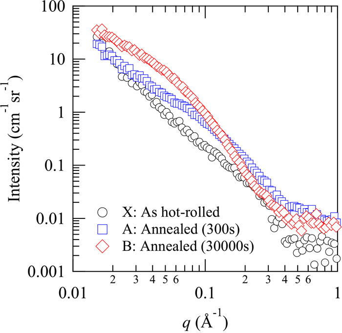
Figure 2 shows the SAXS profiles for the test and reference steels. The difference between the reference steel and the as-hot-rolled steel X is clearly apparent, indicating the occurrence of precipitation already at that stage. With additional annealing, steels A and B exhibited higher scattering intensity than steel X, as clearly observable evidence of the progress of precipitation during annealing. The SAXS profiles include scattering by large scatterers such as inclusions other than TiC precipitates with sizes of several nanometers. Thus, we extracted the actual TiC scattering signal by subtracting the scattering intensity of the reference steel from that of the test steel. Figure 3 shows the SAXS profiles for the test steel samples after subtraction of the reference steel profile. In the SAXS profiles, a smaller q indicates a coarser structure, and the intensity corresponds to the precipitate quantity. In the as-hot-rolled steel X, the precipitate quantity is low and the precipitate size is small, resulting in low scattering intensity. With the progress of the heat treatment from steel A to steel B, in contrast, the profile shifts to the upper left, indicating increase in precipitate size and quantity. The increasing size correlates with the results of the TEM observations.

Fig. 2.

SAXS profiles for steel X, steel A, steel B and reference steel. (Online version in color.)

Fig. 3.

SAXS profiles after subtraction of reference steel profile. (Online version in color.)

Figure 4 shows examples (for steel A) of SAXS profile fitting with a sphere form factor and a disc form factor. With the disc form factor, fitting was performed using the average aspect ratio obtained by TEM. The background,⁴⁾ which has a q⁻⁴ dependence, emerges on the low-q side. This comes from a 50 nm or larger scale structural change and should be excluded in the nanostructure analysis. For the analysis, this contribution is therefore given by the term in the form of C₁q⁻⁴ (C₁: factor of proportionality) in Eq. (1). On the high-q side, a background component not dependent on q appears, which is due to incoherent scattering and other phenomena arising from steel, including X-ray fluorescence. The analysis is performed with this contribution also added to Eq. (1) as a constant term C₂, and Eq. (1)’ is actually used in the analysis:   

$$I(q)=\mathrm{\Delta }{\rho }^{2}Nd\int f(r)V^2(r)F^2(q,r)dr+C_1{q}^{-4}+C_2.$$(1)’

Fig. 4.

SAXS profile for steel A fitted with a) sphere form factor and b) disc form factor. (Online version in color.)

As shown in Fig. 4, the results of fitting were favorable with the assumption of either a sphere or disc form factor. This indicates that when a size distribution is present it is difficult to determine the particle shape from the SAXS profile alone, and direct observation is therefore essential for construction of an accurate structure model. On the other hand, it is also required for SAXS to extract the characteristics of precipitates readily. Thus, it is necessary to understand the difference in results obtained from different models. We therefore performed the following investigation on the effects of models on the results.

Figure 5 shows the TiC sphere equivalent diameter, volume fraction, and number density obtained by fitting with sphere and disc form factors. Here the sphere equivalent diameter is the mean value of the volume fraction density distribution^14,15,16) as the product of the number density coefficient Nd, the volume V(r) and the distribution function f(r), the volume fraction is its integrated value, and the number density is the integrated value of the number density distribution Nd f(r). The TiC sphere equivalent diameter and volume fraction values obtained using the sphere form factor approximately matched those obtained using the disc form factor. The sphere equivalent diameter increased slightly by heat treatment from steel X to steel A, and markedly increased by heat treatment from steel A to steel B. The volume fraction increased markedly by heat treatment from steel X to steel A. The fact that no increase in volume fraction was found between steels A and B, whose values were nearly equal, indicates that the heat treatment at 680°C for 300 s (for steel A) was already sufficient to obtain saturated precipitation. In contrast, the TiC precipitate number density determined as Nd in Eq. (1)’ with sphere and disc form factors differed markedly, by a little less than one order of magnitude. The origin of this difference is discussed in Section 4.3 below. The variation in number density with heat treatment was the same with both form factors. It showed little change in steels X and A but was far lower in steel B.

Fig. 5.

a) Average equivalent diameter, b) volume fraction, c) number density of TiC particles calculated from SAXS profiles. (Online version in color.)

Figure 6 compares the sphere equivalent diameters obtained by TEM observation and by SAXS analysis. The error bars in this figure are not measurement errors, but represent ±1σ for the size distribution. In the SAXS analysis, the standard deviation for each fitting parameter was less than 2%. For steel X and steel A, the TEM and SAXS results were in good agreement, but for steel B the values obtained by SAXS analysis were larger than that obtained by TEM. The reasons for this are discussed in Section 4.2.

Fig. 6.

Average equivalent diameter of TiC particles in test steels obtained by TEM observations and calculated from SAXS profiles with sphere shape and disc shape form factors. Error bars represent ±1σ in size distribution, and not measurement errors. (Online version in color.)

Figure 7 shows the size distributions obtained by TEM and SAXS. Using TEM, sphere equivalent diameters were determined for all observed TiC particles, and their volume-weighted frequency is plotted in the figure. Using SAXS, the volume density distribution Nd V(r) f(r) was calculated and plotted as the size distribution.

Fig. 7.

Histograms of equivalent diameter observed by TEM, and size distributions calculated from SAXS profiles with sphere and disc form factors for a) steel X, b) steel A and c) steel B. (Online version in color.)

For steel X, the size distribution measured using TEM was narrow, whereas all the size distributions determined by SAXS analysis were wide. Other than the differences in spread, the size distributions found by SAXS with the disc form factor were generally close to that found by TEM. In SAXS analysis with the sphere form factor, the obtained distribution was biased toward the left of the size distribution obtained by TEM. The tendency was the same for steel A as for steel X. With the disc form factor, the size distribution was close to that for the TEM observation, but with the sphere form factor the distribution was shifted to the left of the TEM observation results. With regard to steel B, as for the sphere equivalent diameter, the size distribution obtained by SAXS analysis differed markedly from that obtained by TEM observation. For steels X and A, where quantitative results by TEM and SAXS were in good agreement, the size distribution results obtained by SAXS with the disc form factor were found to be close to those obtained by TEM.

4. Discussion

4.1. Validity of Size Distribution Obtained by TEM

Since the SAXS profile is obtained as the sum total of scattering by all scatterers, it is not possible to determine the individual scattering profile for each scatterer. It is therefore difficult to determine the form for each scatterer individually and accurately.

Conversely, if the scatterer shape is given, then the shape of the small-angle scattering profile can be accurately determined by theoretical calculation. The validity of the size distribution obtained from TEM, which is inferior in statistical precision, can therefore be surmised by calculating the scattering profile from the TEM observations and comparing it with the results of the SAXS measurements.

We first calculated the scattering profile for each individual measured TiC particle and then added together the profiles for all of the observed particles. The scattering intensity for the individual particles was calculated using Eq. (4) assuming that they are all randomly orientated. We obtained a sum total profile from the TEM observation results by performing a summation of F²(q, r, t) obtained from Eq. (4) for all particles observed by TEM observation using Eq. (5):⁴⁾   

$$I(q)=\mathrm{\Delta }{\rho }^2\sum V^2(r,t)F^2(q,r,t).$$(5)

Figure 8 shows the results of the calculation for steel A. The profiles shown in blue represent small-angle scattering by individual TiC particles, and the summed profile shown in red can be obtained by adding them all together.

Fig. 8.

Scattering profile for TiC calculated using disc form factor from size of TiC particles observed by TEM in steel A, and profile of summation of all calculated scattering profiles. (Online version in color.)

Figure 9 shows the summed profiles obtained from TEM and the profiles actually determined by SAXS. Note that an accurate number density cannot be determined from the TEM observations and the absolute value of the obtained summed profile is therefore shown with appropriate scale adjustment. For steels X and A, very good agreement was found between the summed profiles determined from TEM observations and the profiles determined from SAXS measurements. The TEM observations yielded profiles matching the SAXS profiles having excellent statistical precision due to large measurement volumes. Thus, it can be considered that the TEM profiles were free from sampling bias and the resulting size distribution can well be regarded as a representative distribution, although the TEM observations were performed locally and the number of TiC particles was at most 95. For steel B, although the two profiles are also roughly in agreement, the degree of coincidence is somewhat inferior, perhaps because of insufficient sampling or bias in the sampling.

Fig. 9.

Measured SAXS profiles after subtraction of reference steel profile, and profiles calculated from size of TiC particles observed by TEM in steel X, steel A and steel B. (Online version in color.)

4.2. Difference between Results of Determination by TEM and SAXS

As shown in Fig. 6, for steel B a large difference was found in average sphere equivalent diameter assessments by TEM and SAXS. One presumable reason for this is a deviation between the lognormal distribution assumed as the size distribution and the actual size distribution.

Figure 10 shows the size distribution quantified by TEM and the results of least squares fitting of the size distribution using the lognormal distribution function. For steels X and A, the size distribution found with TEM was very closely fitted by the lognormal distribution function. The actual TiC size distribution was accordingly close to the lognormal distribution, thus indicating that analysis using a lognormal distribution is essentially problem-free. As shown in Fig. 7, however, the distribution spread obtained by SAXS fitting is wider than that obtained using TEM.

Fig. 10.

Histograms of equivalent diameter observed by TEM, and size distribution fitted with lognormal distribution from histograms in a) steel X, b) steel A, c) steel B. (Online version in color.)

For steel B, the size distribution obtained using TEM diverges substantially from the lognormal distribution, and the divergence from the results in fitting for coarse TiC particles is particularly large. Assuming that the distribution found using TEM is close to the actual distribution, for steel B, one lognormal distribution may be deemed inadequate to describe the size distribution. With such a size distribution, improvement can be obtained by assigning a bimodal, trimodal, or other such size distribution. However, uncertainty tends to emerge as the number of variables increases.

Various problems may thus arise due to inadequacy of the size distribution model. Here we concentrate on the problems that emerged in this investigation and closely examine measures that can be taken against them.

4.3. Divergence in Number Density with Difference in Form Factor

In the SAXS analysis, as shown in Fig. 5, a large difference occurs between the results of number density quantification with sphere and disc form factors. In this section, we discuss the cause of this divergence and methods of finding valid number densities using the results for steels X and A, in which average sphere equivalent diameters determined by SAXS were in good agreement with TEM results.

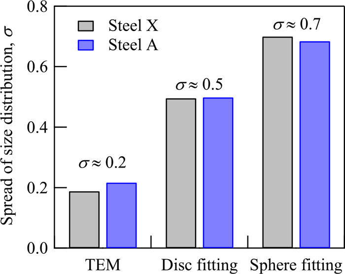
For the sphere equivalent diameter shown in Fig. 7, the distribution obtained with SAXS has a wider spread than that obtained with TEM. Figure 11 shows the value σ, which indicates the spread of the volume density distribution obtained with SAXS and the value of σ obtained by fitting the size distribution measured by TEM with a lognormal distribution. The value based on TEM was approximately σ=0.2 and those obtained in the SAXS analysis were approximately σ=0.5 with the disc form factor and σ=0.7 with the sphere form factor, thus showing that the distribution spread differs with the analysis method.

Fig. 11.

Spread of size distribution σ of TiC particles from TEM observations and SAXS measurements using sphere and disc form factors. (Online version in color.)

Here, as described in Section 4.1, the size distribution found with TEM was considered a representative distribution profile. It is therefore assumed that the TEM analysis yields a σ value close to the actual distribution spread, and the following discussion proceeds on that basis. In the SAXS analysis of plate-like precipitates, fitting by assuming an isotropic particle shape results in a large σ. As plate-like precipitates have two characteristic lengths of thickness and radius, whereas a sphere has just one, compared to the scattering profile for spherical precipitates, the scattering profile for plate-like precipitates appears to have a wider size distribution. If a sphere form factor is used for plate-like precipitates, all such effects of the shape appear in the size distribution, so the value of σ is inevitably overestimated. If the disc form factor is used, in contrast, the effect of the shape is to some degree naturally represented and the value of σ is thus smaller than that using the sphere form factor. In the present analysis, however, the aspect ratio is fixed and the actual shape cannot be completely expressed, and the value of σ is larger than that obtained by TEM analysis.

To investigate the effect of varying σ on the analysis results, with supposition of the volume fraction density distribution Nd V(r) f(r) as the lognormal distribution Λ(1, σ²), we investigated the effect of changing σ alone for a constant volume fraction of precipitates. The volume fraction is held constant because its assessment is considered to be approximately equivalent to evaluating the contribution to the integral scattering intensity for each particle¹⁷⁾ in profile fitting, and the accuracy of the assessment is deemed to be only very slightly dependent on the particle size distribution spread. Another reason for holding the volume fraction constant is because in this investigation the volume fraction was independent of the form factor. Figure 12 shows the calculated distribution functions. For the volume fraction density distribution, the distribution broadened and the peak position shifted to the left with increasing σ. It appears as though the average size is affected by σ because of the change in peak position, but the effect of σ is moderated if the central value (mode) or expected value (mean) is used as the average value. As for the number frequency distribution, the peak position shifts significantly to the left as σ increases and the integrated intensity representing the number density markedly increases in size.

Fig. 12.

Effect of change in spread of size distribution σ for a) volume fraction density and b) number density of particles. (Online version in color.)

In this study, the distribution function f(r) is normalized so that its integral value become 1. The contribution of fine particles to the frequency of the distribution function f(r) markedly increases if σ is large. For the volume fraction density distribution Nd V(r) f(r), since the volume term V(r) acts on f(r), the contribution of fine particles decreases. When Nd is assumed to be constant, the volume fraction V_f, which is the integral of the volume fraction density distribution Nd V(r) f(r), decreases with increasing σ. Since the volume fraction is actually constant, however, the number density coefficient Nd increases to compensate for this. The number density expressed as Nd ∫ f(r) dr = Nd therefore increases with increasing σ.

As shown in Fig. 13, the number density Nd rises sharply with increasing σ. Between σ=0.5, which is equivalent to using the disc form factor, and σ=0.7, which is equivalent to using the sphere form factor, the number density nearly triples. This approximately matches the change in the number density with form factor shown in Fig. 5, thus indicating that in the SAXS analysis the deviation in number density when a sphere or disc form factor is used depends on the difference in size distribution. In summary, if the spread of the distribution is overestimated due to insufficient representation of the precipitate shape, the number density contains computational artifacts, and it should be considered to lack physical validity. Assuming that a distribution spread close to the actual one can be obtained by the TEM method and the σ value is 0.2, the number density obtained by the SAXS analysis is overestimated because the spread of the distribution cannot be correctly evaluated.

Fig. 13.

Effect of spread of size distribution σ for number density of particles. (Online version in color.)

We now proceed to examine the possibility of number density assessment with fairly good accuracy in such cases. The integrated SAXS intensity is proportional to the volume fraction. As described earlier, the accuracy of volume fraction assessment is almost entirely independent of the size distribution spread. From this viewpoint, we define the average number density Nd_ave as   

$$N{d}_{\text{ave}}=\frac{V_f}{V_{\text{ave}}}$$(6)

where V_f is the volume fraction of the precipitates and V_ave is the volume of a precipitate with the average equivalent diameter. The average number density here is for the case where all precipitates have the average equivalent diameter (σ→0). Comparison of the case in Fig. 13, where the TEM equivalent of σ=0.2 can be considered close to the actual value, and the case in which the number density corresponds to the limit σ→0, yields a difference of only 1.2 times. It can therefore be concluded that the average number density is close to the actual value. Accordingly, even if the SAXS analysis yields an overestimate of the size distribution because of a problem in the analysis, a number density close to the actual value can be obtained by incorporating the average number density.

Figure 14 shows the average number densities obtained by SAXS analysis using sphere and disc shape form factors, which are seen to approximately match. This indicates that the effect of overestimation of the size distribution in the SAXS analysis can be eliminated even when the applied shape model is not optimal. Thus, the SAXS analysis can be performed using either a sphere or disc shape factor, and the same quantitative results are obtained for the sphere equivalent diameter, volume fraction, and average number density of precipitates. Even for coherent plate-like precipitates, it has thus been shown that analysis with a convenient, effectively convergent sphere form factor can be used to obtain valid quantitative results. In this report, we ascertained the convenience of the SAXS method and its methodological characteristics in comparison with the widely used method of size assessment by TEM observation, and discussed the possibility of extracting effective quantitative information by simple analysis. In particular, we investigated aspects requiring special care in the use of a lognormal distribution in analysis of particles with shapes other than spherical. The results clearly show that, with due care for these aspects, quantitative parameters can be readily and effectively extracted by a sphere form factor and lognormal distribution analysis, which is the simplest form of SAXS analysis.

Fig. 14.

Average number density and number density of TiC precipitates for steel A and steel B calculated with both sphere and disc form factors. (Online version in color.)

5. Conclusions

In this study, we used SAXS and TEM to quantify coherent plate-like TiC precipitates in steel sheets, and the findings were as follows:

(1) The quantitative values for the TiC average sphere equivalent diameter and the volume fraction found by SAXS analysis with a sphere and disc form factors were found to be in good agreement, and independent of the form factor. However, a large difference was found between the number densities obtained with the two different form factors. For steels X and A, the TiC average sphere equivalent diameters found by SAXS analysis and TEM observations were in good agreement.

(2) When the actual size distribution and the lognormal distribution are greatly different, as in the case of steel B, the quantitative precision of the SAXS analysis clearly decreases. For a sample with a special size distribution of precipitates, if correct assessment of the size distribution is required, it is necessary to provide an actually conforming distribution model.

(3) In the analysis of the plate-like precipitates, the form factor dependence of the number density quantitative results obtained by SAXS was due to overestimation of the size distribution, with which the number density quantitative results became excessive. It was found that, even then, a valid number density can be obtained by using an average number density assuming no distribution spread.

(4) It was shown that for coherent plate-like precipitates such as TiC, valid quantitative results can be obtained conveniently by SAXS analysis using a sphere form factor with good convergence.

References

• 1)   K.  Seto,  Y.  Funakawa and  S.  Kaneko: JFE Tech. Rep., 10 (2007), 19.
• 2)   T.  Murakami,  E.  Kakiuchi,  H.  Hatano,  T.  Arikawa,  H.  Kakimoto and  T.  Choda: Kobe Steel Eng. Rep., 61 (2011), 79 (in Japanese).
• 3)   Y.  Funakawa,  T.  Shiozaki,  K.  Tomita,  T.  Yamamoto and  E.  Maeda: ISIJ Int., 44 (2004), 1945.
• 4)   M.  Ohnuma and  J.  Suzuki: Bull. Iron. Steel Inst. Jpn., 11 (2006), 631 (in Japanese).
• 5)   M.  Ohnuma,  J.  Suzuki,  S.  Ohtsuka,  S.  Kim,  T.  Kaito,  M.  Inoue and  H.  Kitazawa: Acta Mater., 57 (2009), 5571.
• 6)   Y.  Oba,  S.  Koppoju,  M.  Ohnuma,  T.  Murakami,  H.  Hatano,  K.  Sasakawa,  A.  Kitahara and  J.  Suzuki: ISIJ Int., 51 (2011), 1852.
• 7)   Y.  Oba,  S.  Koppoju,  M.  Ohnuma,  Y.  Kinjo,  S.  Morooka,  Y.  Tomota,  J.  Suzuki,  D.  Yamaguchi,  S.  Koizumi,  M.  Sato and  T.  Shiraga: ISIJ Int., 52 (2012), 457.
• 8)   P.  Kozikowski,  M.  Ohnuma,  M.  Ohta,  Y.  Terakado,  Y.  Yoshizawa,  S.  Koppoju and  M.  Lewandowska: Mater. Trans., 58 (2017), 981.
• 9)   R. G.  Baker and  J.  Nutting: Precipitation Processes in Steels, Special report 64, Iron and Steel Institute, London, (1959), 1.
• 10)   H.  Yen,  C.  Chen,  T.  Wang,  C.  Huang and  J.  Yang: Mater. Sci. Technol., 26 (2010), 421.
• 11)   Y.  Tanaka,  K.  Yamada,  Y.  Funakawa and  K.  Sato: Tetsu-to-Hagané, 98 (2012), 84 (in Japanese).
• 12)   F.  Zhang,  J.  Ilavsky,  G.  Long,  J.  Quintana,  A.  Allen and  P.  Jemian: Metall. Mater. Trans. A, 41 (2010), 1151.
• 13)   J. S.  Pedersen: Adv. Colloid Interface Sci., 70 (1997), 171.
• 14)   A. J.  Allen,  D.  Gavillet and  J. R.  Weertman: Acta Metall. Mater., 41 (1993), 1869.
• 15)   A.  Wiedenmann: J. Appl. Crystallogr., 33 (2000), 428.
• 16)   S. M.  He,  N. H.  van Dijk,  M.  Paladugu,  H.  Schut,  J.  Kohlbrecher,  F. D.  Tichelaar and  S.  van der Zwaag: Phys. Rev. B, 82 (2010), 174111.
• 17)  For example,  L. A.  Feigin and  D. I.  Svergun: Structure Analysis by Small-Angle X-ray and Neutron Scattering, Plenum Press, New York, (1987), 46.