Thermodynamic Modeling of Liquid Steel

Abstract

Thermodynamic property of liquid steel is often described by activity coefficient of solute in the steel (the other form of partial excess Gibbs energy of the solute). Reliable description of the activity coefficient is required in order to predict equilibrium content of the solute as accurately as possible. In the present article, a number of such approaches are reviewed, with emphases on basic assumption and inherent character of each formalism/model, and on its applicability at high alloyed liquid steel. Chemical interaction between elements was categorized as weak interaction (i.e., between metal and metal) and strong interaction (i.e., between metal and non-metal). Each formalism/model was analyzed in the view of thermodynamic consistency (Gibbs-Duhem equation and Maxwell’s relation). It is concluded that two issues should be explicitly and simultaneously considered: obeying thermodynamic consistency and treating strong chemical interaction. The former ensures its applicability at higher solute content, and the latter is necessary to properly handle the strong interaction between metallic elements and non-metallic elements, contrary to conventional random mixing assumption.

1. Introduction

This article provides a review of thermodynamic descriptions (theoretical model and formalism) of liquid steel which is basically an Fe based multicomponent liquid alloy. This is an extension of excellent thermodynamic analyses of liquid alloy by Darken,^1,2) Schuhmann Jr.,³⁾ and Pelton.⁴⁾ Several thermodynamic models and formalisms have been used to calculate equilibrium solubility of various elements in steel in contact with other phases (gas, inclusion, slag, refractory, etc.). This article does not intend to provide a parameter set of particular model/formalism, but to show inherent character of the model/formalism as simple as possible. Moreover, beyond typical applications of those model/formalism confined in dilute region of liquid steel, it is also intended to discuss capability of those at higher content of elements in the steel. This would be useful when high alloyed steel such as TRIP, TWIP, and lightweight steel is developed.

Thermodynamic property of liquid steel has been often treated by formulating activity coefficient of component (γ_i) in liquid steel:   

$${\gamma }_i=\frac{a_i}{X_i}$$(1)

where a_i and X_i are the activity and the atom fraction of the component i. a_i and γ_i are partial properties of Gibbs energy of the liquid steel via:   

$$g_i=g_i^{\circ }+\text{R}Tln{a}_i=g_i^{\circ }+\text{R}Tln{\gamma }_i+\text{R}Tln{X}_i$$(2)

  

$$={\frac{\partial G}{\partial n_i})}_{n_j\ne n_i}$$(3)

where G, g_i, $g_i^{\circ }$, R, and T are the Gibbs energy of the steel, the partial Gibbs energy of the component i, the molar standard Gibbs energy of the i, gas constant, and temperature, respectively. Standard state of a_i and γ_i depend on the choice of $g_i^{\circ }$. Activity is often expressed in terms of mass pct. base (a_i = f_i [% i]) for practical purpose, but the Eq. (1) will be used throughout this article for the purpose of this review.

The activity coefficients (γ_i or f_i) have been usually expressed as functions of composition and temperature. These are then used to calculate equilibrium content of each element under controlled activity in equilibrium with other phases. For example, a deoxidation equilibria in liquid steel by Al can be analyzed by:   

$$\mathrm{A}{\mathrm{l}}_2{\mathrm{O}}_3\left(\mathrm{s}\right)=2\underset{\_}{\mathrm{A}\mathrm{l}}+3\underset{\_}{\mathrm{O}};K_{(4)}$$(4)

  

$$K_{\left(4\right)}=\frac{a_{\text{Al}}^2{a}_{\text{O}}^3}{a_{{\text{Al}}_2{\text{O}}_3}}=\frac{{\gamma }_{\text{Al}}^2{\gamma }_{\text{O}}^3{X}_{\text{Al}}^2{X}_{\text{O}}^3}{a_{{\text{Al}}_2{\text{O}}_3}}$$(5)

At a given K₍₄₎ and $a_{{\text{Al}}_{\text{2}}{\text{O}}_{\text{3}}}$, X_Al and X_O are determined if γ_Al and γ_O are known. Accurate description of the γ_i is thus important. Therefore, in this article, emphases are given to the followings:

· thermodynamic consistency of models and formalisms

· applicability of the models and the formalisms to higher content beyond dilute region

· ability of the models and the formalisms in treating of strong interaction among components

Throughout this article, components of liquid steel are designated by 1, 2, ∙∙∙, N-1, and N (1 is a solvent) or Fe–M–X where M is a metallic component and X is a non-metallic component.

G (or G^ex) stands for total energy (or the excess Gibbs energy) of the steel in J, while g (or g^ex) stands for the molar Gibbs energy (or the molar excess Gibbs energy) in J mol⁻¹. γ_i can be obtained either from G^ex or g^ex via:   

$$\text{R}Tln{\gamma }_i=g_i^{\text{ex}}={\frac{\partial G^{\text{ex}}}{\partial n_i})}_{n_j\ne n_i}=g^{\text{ex}}+{\sum }_{j=2}^N\left({\delta }_{ij}-X_j\right)\frac{\partial g^{\text{ex}}}{\partial X_j}$$(6)

where δ_ij is the Krönecker delta. The γ_i is expressed either by an explicit form for the γ_i itself or is obtained by differentiating the (molar) excess Gibbs energy by the Eq. (6), which may not give an explicit form of composition.

Liquid steel is an Fe-based multicomponent liquid alloy. Typical elements of liquid steel are listed in Table 1. These elements may be classified by the following characters:

· metallic vs non-metallic

· stable as condensed phase (liquid or solid) vs stable as gas phase at steelmaking temperature

· attractive to Fe vs repulsive to Fe

Table 1. Major elements M in liquid steel, enthalpy of mixing of binary Fe–M liquid alloy (with respect to the stable phase at 1600°C), and a self-interaction parameter ${\epsilon }_{\text{M}}^{\text{M}}$.¹⁴⁾ g, l, and s in parentheses refer to gas, liquid, and solid indicating a stable form of the element at steelmaking temperature. “+” means strong positive deviation, yielding an immiscibility in the liquid.

M

O(g)

S(g)

P(g)

Si(l)

B(l)

Al(l)

Ti(l)

Ta(s)

Nb(s)

V(s)

Y(l)

W(s)

Ni(l)

Cr(s)

ΔH (kJ mol−1)

−230

−68

−48

−42

−33

−21

−19

−14

−13

−9

−8

−5

−5

−4

${\epsilon }_{\text{M}}^{\text{M}}$

−12.5

−3.3

8.4

13.2

2.5

5.6

2.7

−0.7

0.2

0

M

Mo(s)

Mn(l)

Ce(l)

La(l)

N(g)

Sn(l)

Cu(l)

Zn(g)

C(s)

H(g)

Mg(g)

Ca(g)

Pb(g)

ΔH (kJ mol−1)

−3

−1

−1

0

7

8

16

+

+

+

+

${\epsilon }_{\text{M}}^{\text{M}}$

0

0.8

7.1

6

6.6

1

H, B, C, N, O, P, S are regarded as the non-metallic elements among the components listed in the Table 1. H, N, O, P, S as well as Ca, Mg, Pb, Zn vaporize at temperature of steelmaking. Therefore, solubility of these elements in liquid steel are generally low. Interaction with Fe (either attractive or repulsive) was characterized by the enthalpy of mixing (ΔH). Among those elements, O shows the most negative ΔH, representing very strong attraction to Fe. On the other hand, Ca and Mg are known to form wide immiscibility with Fe, although accurate ΔH could not be measured due to its volatile character. In general, non-metallic element exhibits strong attraction to Fe (and other metals), although some exceptions are found (H, N). The strong attraction between elements requires careful description of the activity coefficient (or excess Gibbs energy), due to significant deviation from random mixing behavior of atoms.

2. Interaction Parameter Formalism

Chipman and coworker noticed that activity coefficient of a solute in liquid steel depends on significantly by C content.^5,6,7,8,9) For example, 2 mass pct. of C increases the activity coefficient of Si by 2 times. This necessitates a formulation of the activity coefficient as a function of composition (apart from temperature). Wagner employed a Taylor series expansion for the ln γ_i.¹⁰⁾ This yields a well-known Wagner’s Interaction Parameter Formalism (WIPF):   

$$\begin{array}{l}ln{\gamma }_i={(ln{\gamma }_i)}_{X_i\to 0}+{\sum }_{j=2}^N{\left(\frac{\partial ln{\gamma }_i}{\partial X_j}\right)}_{X_i,X_j\to 0}{X}_j+\cdots \\ \hspace{1em}\hspace{1em}=ln{\gamma }_i^{°}+{\sum }_{j=2}^N{\epsilon }_i^j{X}_j+\cdots \end{array}$$(7)

where ${\gamma }_i^{\circ }$ and ε_i^j are the Henrian activity coefficient of the i, and the first-order interaction parameter.

Using the Maxwell relations, Wagner showed that:   

$${\epsilon }_i^j={\epsilon }_j^i$$(8)

at infinite dilution.¹⁰⁾ When the experimental data were measured with high accuracy, the second order interaction parameters (ρ_i^j, ρ_i^j,k) were evaluated:¹¹⁾   

$$ln{\gamma }_i=ln{\gamma }_i^{°}+{\sum }_{j=2}^N{\epsilon }_i^j{X}_j+{\sum }_{j=2}^N{\rho }_i^j{X}_j^2+{\sum }_{\begin{array}{c}j=2,k=2\\ j\ne k\end{array}}^N{\rho }_i^{j,k}{X}_j{X}_k+\cdots$$(9)

Extensive literature survey resulted in a compilation of the interaction parameters.^12,13,14)

It is stressed that the evaluation of each parameter was performed independently giving the best fit to the experimental data within limited composition and temperature range. Since this is a mathematical formalism based on the fact that the γ_i should be a function of composition^5,6,8,9) at a given temperature, it does not ensure that the γ_i of the WIPF obeys thermodynamic consistency condition, as will be discussed in Sec. 4.1.^{1,3,4,;15,16,17, 18,19,20,21,22,23,24,25)} Although its definition is strictly valid for the limiting case (X_i → 0 for all i),¹⁰⁾ it has been often used at finite content with some success. Although it is easy to use and widely applied in metallurgical community, its validity is somewhat limited. It often fails in calculation of equilibrium content of solutes in liquid steel, when it contains strong deoxidizer or is applied to higher solute content. In the following sections, further efforts to overcome this shortcoming of WIPF are reviewed. In order to deliver the content of the present article efficiently, characteristics of the activity coefficients of various solutes in liquid steel are introduced in advance.

3. Characteristic of Thermodynamic Properties of Liquid Steel

3.1. Changes of γ_i by Composition Change

In 1–2 binary system showing negative deviation, the γ₂ is less than unity. It increases as X₂ increases, and approaches to the unity at X₂ = 1 (Raoult’s law). Most simple and natural increase of the ln γ₂ may be represented schematically in Fig. 1(a) (Case I). The ln γ₂ increases monotonously as X₂ increases. This may be represented by a simple regular solution model:   

$$g^{\text{ex}}={\omega }_{12}{X}_1{X}_2$$(10)

with an interaction energy ω₁₂ < 0. The ln γ₂ is obtained using the Eq. (6):   

$$ln{\gamma }_2=\frac{{\omega }_{12}}{\text{R}T}{(1-X_2)}^2={\alpha }_{12}{(1-X_2)}^2$$(11)

where α₁₂ is the interaction parameter (no unit). The corresponding g^ex may be seen in Fig. 1(b). A parabolic shape is identified. Darken’s excess stability:¹⁾   

$$\Psi =\frac{d^2{g}^{\text{ex}}}{d{X}_2^2}=\frac{1}{1-X_2}\text{R}T\frac{dln{\gamma }_2}{d{X}_2}$$(12)

is also shown in Fig. 1(c). According to Darken,¹⁾ a strong attraction between the two components yields a pronounced peak on a Ψ, which may also appear as an intermediate solid phase in the 1–2 binary phase diagram. In Fig. 1(c), no such peak is seen. Therefore, the interaction between 1–2 in the Case I is weak, close to random mixing of the two components. The g^ex is proportional to X₁X₂, which is a half of the probability of finding 1–2 pair in the random mixing solution.

Fig. 1.

Activity coefficient, excess Gibbs energy, and excess stability of 1–2 binary solution: (a)–(c) weak interaction between 1 and 2, (d)–(f) strong interaction between 1 and 2, (g)–(i) strong interaction between 1 and 2, with a repulsion between 1 and “12”.

When the interaction becomes stronger (Case II), the ln γ₂ increases as X₂ increases, but somewhat in different manner, as seen in Fig. 1(d): the ln γ₂ increases moderately at low X₂, then increases suddenly at a particular composition (X₂ = ~0.5 in this example), followed by approaching moderately to zero (by the Raoult’s law). This is interpreted as follows. Adding small amount of 2 in pure 1 results in strong ordering of the 2. This lowers the activity of 2 compared to that in a weak interacting system (or random mixing solution). Therefore, the ln γ₂ increases only slightly while X₂ increases. This continued up to the composition of maximum ordering where the solvent 1 could bind 2 as much as possible. Over this composition, additionally added 2 becomes free from the binding by 1, thereby a₂ increases as if 2 were in an ideal solution (ln γ₂ = ~0). The strong ordering at low X₂ results that g^ex (mostly enthalpy of mixing) changes as much as 2 enters in the solution. Contrary to the parabolic shape (Fig. 1(b)), a sharp decrease of the g^ex is expected (linearly proportional to X₂), yielding a “V-shape” (Fig. 1(e)). This is consistent with the “titration-like” curve of the ln γ₂ (Fig. 1(d)). Corresponding Ψ shows a pronounced peak near X₂=0.5, implying a strong ordering at the composition (Fig. 1(f)).

Both two cases (Case I and Case II) are representing negative deviation, therefore ln ${\gamma }_2^{\circ }$ < 0 and ${\epsilon }_2^2$ > 0. In Table 1, B, Al, Si, P, Ti, Ni fall in this category (ΔH < 0, ${\epsilon }_2^2$ > 0). On the other hand, in case of O and S exhibiting very negative ΔH, ${\epsilon }_2^2$ is also negative. Such cases are represented schematically in Fig. 1(g) (Case III). This observation shows that sign of the ${\epsilon }_2^2$ does not reflect the type of interaction between 1 and 2 (attraction or repulsion). Having ${\epsilon }_2^2$ < 0 requires an inflection point on g^ex (see Fig. 1(h)). This is based on the fact that although the attraction between the components 1 and 2 is very strong, the component 1 (with dilute 2) and the component 2 (already coupled with the component 1) has a strong repulsion. The Case II and Case III are hardly reproduced by WIPF, over wide composition range.

3.2. Phase Diagram and Interaction Parameter

Change of the activity coefficient may be qualitatively read from the phase diagram. Figure 2 shows phase diagrams of Fe–P, Fe–S, and Fe–O binary systems (Fe: 1, P/S/O: 2 in the above analysis). P, S, and O exhibit very strong attraction to Fe (ΔH < 0), thereby yielding negative deviation (γ₂ < 1), as listed in the Table 1. ${\epsilon }_{\mathrm{P}}^{\mathrm{P}}$ > 0, corresponding the Case I or more likely Case II. In Fig. 2(a), liquidus of α-bcc phase decreases monotonously as X_P increases up to the eutectic point: adding P to liquid Fe results in strong and natural negative deviation. On the other hand, in Fe–S system, ${\epsilon }_{\mathrm{S}}^{\mathrm{S}}$ is negative, corresponding to the Case III. Figure 2(b) shows that the liquidus of α-bcc/γ-fcc decreases as X_S increases, however the liquidus exhibits an inflection point. This reflects metastable immiscibility in the liquid (shown by a dashed curve), as a result of the repulsion between Fe (with very low S) and S (coupled with Fe). In case of Fe–O binary system, stronger attraction between Fe and O and stronger repulsion between Fe (with very low O) and O (coupled with Fe) result in considerably negative ΔH and ${\epsilon }_{\mathrm{O}}^{\mathrm{O}}$. A stable miscibilty gap between liquid Fe and liquid FeO is seen in Fig. 2(c).

Fig. 2.

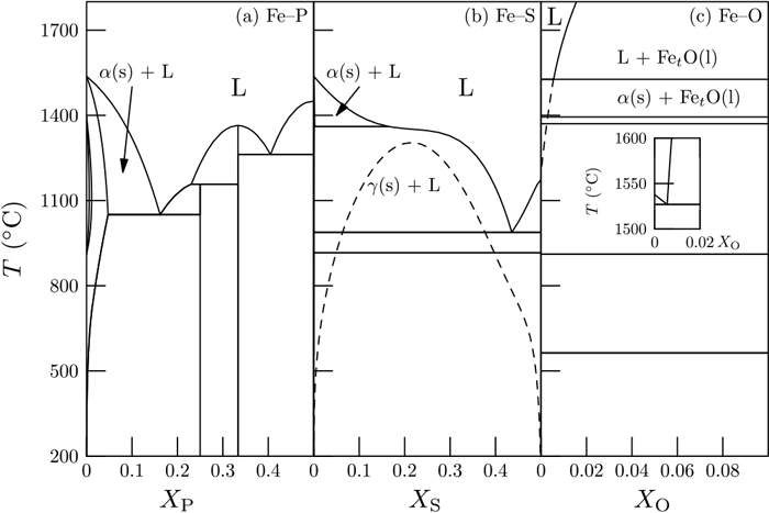
Binary phase diagram of (a) Fe–P, (b) Fe–S, and (c) Fe–O (with an inset of a part of the phase diagram near the melting temperature of Fe) systems.

The activity coefficient of components in liquid steel is basically a result of thermodynamic characteristic of chemical interaction between the components (not only with Fe but also with other solutes). Different signs of ${\epsilon }_2^2$ of very strongly attracting systems are indeed results of complicated interactions (simple but strong attraction in some cases such as Fe–P giving positive ${\epsilon }_{\mathrm{P}}^{\mathrm{P}}$ vs simultaneous attraction and repulsion in some cases such as Fe–S or Fe–O system giving negative ${\epsilon }_{\mathrm{S}}^{\mathrm{S}}$ and ${\epsilon }_{\mathrm{O}}^{\mathrm{O}}$). As seen in the Fig. 1, the strongly interacting system exhibits complicated curvature in the ln γ₂, which may not be simply described by a simple polynomial function. In order to calculate equilibrium content of components in liquid steel accurately, the activity coefficients of the components should be accurately evaluated. In the following section, a review of various approaches in the calculation of activity coefficient in liquid steel is presented.

4. Weak Interaction: Fe – M

4.1. Darken’s Quadratic Formalism

Darken identified some regularities of ln γ₁ and ln γ₂ in a terminal region in 1(solvent)–2(solute) binary liquid solution. At a given T, he found that the ln γ₁ is adequately represented by the following equation:   

$$ln{\gamma }_1={\alpha }_{12}{X}_2^2$$(13)

When the Gibbs-Duhem equation   

$${\sum }_{i=1}^N{X}_{i}dln{\gamma }_i=0$$(14)

is applied for N = 2, it gives   

$$ln{\gamma }_2={\alpha }_{12}{(1-X_2)}^2+I_{12}$$(15)

where I₁₂ is an integration constant. Many binary systems show the ln γ₂ often obey this quadratic form. Figure 3 shows various examples of the regularity.^{26,27,28,29,30,31,32,33,34)} The Eq. (15) is rearranged as:   

$$ln{\gamma }_2=\left({\alpha }_{12}+I_{12}\right)-2{\alpha }_{12}{X}_2+{\alpha }_{12}{X}_2^2$$(16)

Fig. 3.

Darken’s plot for the activity coefficient of 2 (= Al,²⁶⁾ Cu,²⁷⁾ Mn,²⁸⁾ Ni,^29,30) Si^31,32,33,34)) in 1–2 binary liquid alloys at 1600°C (except Fe–Cu at 1550°C, 1 = Fe). (Online version in color.)

The above expression is inherently a second order interaction parameter formalism. However, contrary to the WIPF, the first- and second-order parameters are interdependent. When the Eq. (16) is compared to the Eq. (9) in the 1–2 binary system, (α₁₂ + I₁₂) corresponds to ln ${\gamma }_2^{\circ }$, α₁₂ corresponds to −1/2 ${\epsilon }_2^2$ = ${\rho }_2^2$. When X₂ approaches to zero, the Eq. (16) reduces to the first-order equation of WIPF.¹⁰⁾ At higher X₂, Darken’s formalism inherently considers the quadratic term. It should be noted that when I₁₂ = 0, Darken’s quadratic formalism reduces exactly to a well-known regular solution model. From the Eqs. (13) and (16) with (α₁₂ + I₁₂) = ln ${\gamma }_2^{\circ }$, the molar excess Gibbs energy of the 1–2 system is obtained as:   

$$g^{\text{ex}}=\text{R}T\left(X_{1}ln{\gamma }_1+X_{2}ln{\gamma }_2\right)=\text{R}T\left(X_{2}ln{\gamma }_2^{°}-{\alpha }_{12}{X}_2^2\right)$$(17)

Darkens extended his quadratic formalism to a ternary 1–2–3 system:²⁾   

$$\begin{array}{l}{g}^{\text{ex}}=\text{R}T[X_{2}ln{\gamma }_2^{°}+X_{3}ln{\gamma }_3^{°}-{\alpha }_{12}{X}_2^2-{\alpha }_{13}{X}_3^2\\ \hspace{1em}\hspace{0.5em}-\left({\alpha }_{12}+{\alpha }_{13}-{\alpha }_{23}\right)X_2{X}_3]\end{array}$$(18)

The last term was specially designed in order to yield a ternary regular solution model:   

$$\begin{array}{l}{g}^{\text{ex}}=\text{R}T\left({\alpha }_{12}{X}_1{X}_2+{\alpha }_{13}{X}_1{X}_3+{\alpha }_{23}{X}_2{X}_3\right)\\ \hspace{1em}\hspace{0.5em}={\omega }_{12}{X}_1{X}_2+{\omega }_{13}{X}_1{X}_3+{\omega }_{23}{X}_2{X}_3\end{array}$$(19)

when I₁₂ = I₁₃ = 0 (ln ${\gamma }_2^{\circ }$ = α₁₂ and ln ${\gamma }_3^{\circ }$ = α₁₃). By substituting the Eq. (19) into the Eq. (6), the ln γ₁, ln γ₂, and ln γ₃ are obtained.   

$$ln{\gamma }_1={\alpha }_{12}{X}_2^2+{\alpha }_{13}{X}_3^2+\left({\alpha }_{12}+{\alpha }_{13}-{\alpha }_{23}\right)X_2{X}_3$$(20)

  

$$\begin{array}{l}ln\left({\gamma }_2/{\gamma }_2^{°}\right)=-2{\alpha }_{12}{X}_2+\left({\alpha }_{23}-{\alpha }_{12}-{\alpha }_{13}\right)X_3+{\alpha }_{12}{X}_2^2+{\alpha }_{13}{X}_3^2\\ \hspace{1em}\hspace{1em}\hspace{1em}\hspace{1em}\hspace{0.5em}+\left({\alpha }_{12}+{\alpha }_{13}-{\alpha }_{23}\right)X_2{X}_3\end{array}$$(21)

  

$$\begin{array}{l}ln\left({\gamma }_3/{\gamma }_3^{°}\right)=-2{\alpha }_{13}{X}_3+\left({\alpha }_{23}-{\alpha }_{12}-{\alpha }_{13}\right)X_2+{\alpha }_{12}{X}_2^2+{\alpha }_{13}{X}_3^2\\ \hspace{1em}\hspace{1em}\hspace{1em}\hspace{1em}\hspace{1em}+\left({\alpha }_{12}+{\alpha }_{13}-{\alpha }_{23}\right)X_2{X}_3\end{array}$$(22)

When the Eqs. (20), (21), (22) are compared to the Eq. (9) in the 1–2–3 ternary system, it is easily seen that:   

$$-\frac{1}{2}{\epsilon }_2^2={\rho }_2^2={\rho }_3^2={\alpha }_{12}$$(23)

  

$$-\frac{1}{2}{\epsilon }_3^3={\rho }_3^3={\rho }_2^3={\alpha }_{13}$$(24)

  

$${\epsilon }_2^3={\epsilon }_3^2=-{\rho }_2^{2,3}=-{\rho }_3^{2,3}={\alpha }_{23}-{\alpha }_{12}-{\alpha }_{13}$$(25)

From the above relations, it can be seen that the interaction parameters (ε_i^j, ρ_i^j, ρ_i^j,k) are indeed dependent each other. Lupis and Elliott provided more general relationships among the interaction parameters.¹¹⁾ From the above analysis, it is evident that

· I₁₂ and I₁₃ must be zero if the above formalism is to be valid even at X₂ → 1 (and X₃ → 1).

· the Eqs. (23), (24), (25) should be satisfied in order for this formalism to be thermodynamically consistent.

Darken claimed that WIPF is not thermodynamically consistent except at infinite dilution.¹⁾ This has been well appreciated by numerous publications.^{3,4,15,16,17,18,19,20,21,22,23,24,25)} For the activity coefficient as the partial excess Gibbs energy, the Gibbs-Duhem equation must be satisfied:   

$$X_{1}dln{\gamma }_1+X_{2}dln{\gamma }_2+X_{3}dln{\gamma }_3=0$$(26)

Also, the following equation must satisfy in order to fulfill the thermodynamic consistency in 1–2–3 ternary solution:²⁾   

$$\left(1-X_3\right)\frac{\partial ln{\gamma }_2}{\partial X_3}+X_3\frac{\partial ln{\gamma }_3}{\partial X_3}=X_2\frac{\partial ln{\gamma }_2}{\partial X_2}+\left(1-X_2\right)\frac{\partial ln{\gamma }_3}{\partial X_2}$$(27)

This is basically obtained by the Maxwell relation:   

$$\frac{\partial }{\partial n_3}\left(\frac{\partial G^{\text{ex}}}{\partial n_2}\right)=\frac{\partial }{\partial n_2}\left(\frac{\partial G^{\text{ex}}}{\partial n_3}\right)$$(28)

The two Eqs. (26) and (27) must be satisfied for the activity coefficients in the 1–2–3 ternary solution in order to keep thermodynamic consistency condition.²⁾

4.2. Unified Interaction Parameter Formalism

Using the Eqs. (23), (24), (25), the Eqs. (20), (21), (22) can be rewritten as¹:   

$$ln{\gamma }_1=-\frac{1}{2}{\epsilon }_2^2{X}_2^2-\frac{1}{2}{\epsilon }_3^3{X}_3^2-{\epsilon }_2^3{X}_2{X}_3$$(29)

  

$$ln\left({\gamma }_2/{\gamma }_2^{°}\right)={\epsilon }_2^2{X}_2+{\epsilon }_2^3{X}_3+\left(-\frac{1}{2}{\epsilon }_2^2{X}_2^2-\frac{1}{2}{\epsilon }_3^3{X}_3^2-{\epsilon }_2^3{X}_2{X}_3\right)$$(30)

  

$$ln\left({\gamma }_3/{\gamma }_3^{°}\right)={\epsilon }_3^2{X}_2+{\epsilon }_3^3{X}_3+\left(-\frac{1}{2}{\epsilon }_2^2{X}_2^2-\frac{1}{2}{\epsilon }_3^3{X}_3^2-{\epsilon }_2^3{X}_2{X}_3\right)$$(31)

The terms in the parentheses are identical to the ln γ₁, regardless of the solutes. It is to be noted that the activity coefficient of solvent was not considered in WIPF. Pelton and Bale recognized that if one wants to use the Eq. (9) but in a thermodynamically correct way, the second-order terms in the Eq. (9) should be formulated as seen in the Eqs. (30) and (31).^35,36) This is indeed the same as adding the ln γ₁ to the ln γ₂ (and the ln γ₃) of the first-order term (first two terms in the Eq. (9)):   

$$ln{\gamma }_2=ln{\gamma }_2^{°}+{\epsilon }_2^2{X}_2+{\epsilon }_2^3{X}_3+\text{ln}{\gamma }_1$$(32)

  

$$ln{\gamma }_3=ln{\gamma }_3^{°}+{\epsilon }_3^2{X}_2+{\epsilon }_3^3{X}_3+\text{ln}{\gamma }_1$$(33)

They showed that the Eqs. (32) and (33) satisfies the Gibbs-Duhem equation (Eq. (26) with the ln γ₁ (Eq. (29)) and the Maxwell relation (27). This ensures necessary and sufficient thermodynamic consistency, and eliminates the errors in the WIPF. Moreover, well evaluated first-order interaction parameters of the WIPF can be directly used without any conversion.^12,13,14) They call this formalism as Unified Interaction Parameter Formalism (UIPF), because this unifies the WIPF at the infinite dilution, Lupis and Elliott’s second order formalism, Darken’s formalism at higher solute content.

The UIPF can be expanded to include second-order parameters (ε_ijk in the notation of Pelton and Bale^4,35,36)) or higher-order parameters for the activity coefficient of solutes in 1–2–∙∙∙–N multicomponent solution. This satisfies the Gibbs-Duhem equation in the N–component system (Eq. (14)) and the Maxwell relation such as the Eq. (28) for all solutes i and j (i, j = 2, ∙∙∙, N).

Pelton and Bale proposed that the addition of ln γ₁ to the conventional WIPF is the way of correction of the Wagner’s formalism to be thermodynamically consistent.^4,35,36) This ensures that the application of interaction parameter formalism even at higher content of solutes is thermodynamically correct.

Malakhov raised a possibility that there may be infinite number of ways of such correction to the WIPF, which can satisfy both the Gibbs-Duhem equation (Eq. (26)) and the Maxwell relation (Eq. (27)) in 1–2–3 ternary solution.²⁴⁾ However, recently, the present author pointed out that considering the Maxwell relation not only between solute-solute but also between solvent-solute resolves the issue raised by Malakhov, and concluded that the correction made by Pelton and Bale is the only way of such corrections.²⁵⁾ The present author extended the Eq. (27) to the N-component system including the solvent-solute interaction:   

$${\sum }_{k=2}^N\left({\delta }_{ik}-X_k\right)\frac{\partial ln{\gamma }_j}{\partial X_k}={\sum }_{k=2}^N\left({\delta }_{jk}-X_k\right)\frac{\partial ln{\gamma }_i}{\partial X_k}$$(34)

where i and j are 1 (solvent), 2, ∙∙∙, N. This must be obeyed by all the ln γ_i to be thermodynamically consistent, apart from the Eq. (14).

Miki and Hino applied the Darken’s quadratic formalism to interpret deoxidation phenomena in high alloyed steel.^{37,38,39,40,41,42,43,44)} They expanded the interaction energy (ω_ij) using Redlich-Kister type polynomial.⁴⁵⁾ This yields essentially identical formalism to the UIPF up to higher order, or the proposal by Hillert using a modified regular solution model for terminal solution.⁴⁶⁾

¹  Pelton and Bale used ε_ij, instead of ε_i^j.^4,35,36)

4.3. Regular Solution for Dilute Component X

Consider that a non-metallic component X dissolves in a binary Fe–M metallic liquid solution (Fe–M–X). As mentioned in Sec. 1, interaction between Fe–M is generally weaker than that between Fe–X and M–X. Alcock and Richardson treated the dissolution of the X in the Fe–M binary solution in a pairwise manner, and counted number of pairs and associated energy change upon the dissolution.⁴⁷⁾ They derived the following equation for the Henrian activity coefficient of infinitely dilute solution of X (${\gamma }_{\mathrm{X}}^{°}$) in Fe–M:   

$$ln{\gamma }_{\text{X}}^{°}=X_{\text{Fe}}ln{\gamma }_{\text{X}\left(\text{Fe}\right)}^{°}+X_{\text{M}}ln{\gamma }_{\text{X}\left(\text{M}\right)}^{°}-X_{\text{Fe}}{X}_{\text{M}}{\alpha }_{\text{FeM}}$$(35)

where ${\gamma }_{\text{X}\left(\text{Fe}\right)}^{°}$, ${\gamma }_{\text{X}\left(\text{M}\right)}^{°}$, and α_FeM are the Henrian activity coefficient of X in pure liquid Fe, that in pure liquid M, and the interaction parameter between Fe and M, respectively. This can also be simply obtained by setting 1 = Fe, 2 = M, 3 = X in the Eq. (19), differentiating it to get the partial excess Gibbs energy X:   

$$ln{\gamma }_X=X_{\text{Fe}}\left(1-X_{\text{X}}\right){\alpha }_{\text{FeX}}+X_{\text{M}}\left(1-X_{\text{X}}\right){\alpha }_{\text{MX}}-X_{\text{Fe}}{X}_{\text{M}}{\alpha }_{\text{FeM}}$$(36)

and by setting:   

$$ln{\gamma }_{\text{X}\left(\text{Fe}\right)}^{°}=\underset{X_{\text{X}}\to 0}{\text{lim}}{\alpha }_{\text{FeX}}{(1-X_{\text{X}})}^2={\alpha }_{\text{FeX}}$$(37)

  

$$ln{\gamma }_{\text{X}\left(\text{M}\right)}^{°}=\underset{X_{\text{X}}\to 0}{\text{lim}}{\alpha }_{\text{MX}}{(1-X_{\text{X}})}^2={\alpha }_{\text{MX}}$$(38)

in the limit of X_X → 0. By the general definition of Wagner’s interaction parameter (Eq. (7)), the first-order interaction parameter is obtained as:   

$${\epsilon }_{\text{X}}^{\text{M}}=\frac{\partial ln{\gamma }_X}{\partial X_{\text{M}}}{)}_{X_{\text{M}}\to 0,\mathrm{\hspace{0.17em} }{X}_{\text{X}}\to 0}=ln{\gamma }_{\text{X}\left(\text{M}\right)}^{°}-ln{\gamma }_{\text{X}\left(\text{Fe}\right)}^{°}-{\alpha }_{\text{FeM}}$$(39)

The Eq. (39) is indeed equivalent to the Eq. (25). The Eq. (35) can be easily extended to multi-component 1–2–∙∙∙– (N−1) –X.⁴⁷⁾

4.4. Discussion

It can be concluded that Darken’s formalism in Sec. 4.1,^1,2) Unified Interaction Parameter Formalism in Sec. 4.2,^4,35,36) Hillert’s modified regular solution model,⁴⁶⁾ and Alcock and Richardson’s regular solution model in Sec. 4.3⁴⁷⁾ are essentially identical inasmuch as these are all based on the well known regular solution theory. Darken’s starting point (Eq. (13)) indeed conforms with the regular solution theory, of which the energy change is basically described by pairwise interaction. It should be stressed that in this theory, a probability of finding a nearest pair of (i–j) is 2X_iX_j when i ≠ j or X_i² when i = j. This is equivalent to say that the atoms i and j are distributed randomly over a quasi-lattice, regardless of the size of interaction energy ω_ij (or α_ij). It is evident that the interaction between metal and non-metal cannot be successfully described assuming such näive random mixing concept. Alcock and Richardson found that their model (Eq. (35)) works well when a difference between ln ${\gamma }_{\text{X}\left(\text{Fe}\right)}^{°}$ and ln ${\gamma }_{\text{X}\left(\text{M}\right)}^{°}$ is less than unity.⁴⁸⁾ However, the ${\epsilon }_{\text{X}}^{\mathrm{M}}$ calculated by the Eq. (39) was correct in sign, but was smaller than available experimental data.⁴⁹⁾ For example, ${\epsilon }_{\text{O}}^{\mathrm{A}1}$ calculated by the Eq. (39) was 90 times smaller that the experimental data.⁴⁹⁾ This is due to neglecting the strong Short-Range Ordering (SRO) between Al and O, as already pointed out by themselves.⁴⁸⁾ Such discrepancy is well identified in a liquid steel when an alloying element M reacts with a non-metal element such as O. Figure 4 shows ln γ_O in liquid Fe–M–O alloys (M = Al or Mn) as a function of X_M, extracted from available deoxidation experimental data.^{50,51,52,53,54,55) 2} As X_M increases, the ln γ_O gradually decreases. If the WIPF is used (Eq. (9)), the ln γ_O must be expressed with higher order terms, at least second-order terms. Since formalism and models discussed in this section are thermodynamically consistent and those are indeed identical, Darken’s formalism (Eqs. (21) and (22)) was used to test how ln ${\gamma }_{\mathrm{X}}^{°}$ varies as a function of X_M in an example Fe–M–X system³. Figure 5 shows the calculated results with various α_FeM. In this test calculation, α_FeX and α_MX were arbitrarily set to 0 and −15, respectively, which results in a similar scale to those in Fig. 4(a). I_FeM and I_FeX were set to zero. Depending on the α_FeM, composition dependence of the ln ${\gamma }_{\mathrm{X}}^{°}$ varies. However, in order to have a similar composition dependence as those seen in the Fig. 4 at least qualitatively, it requires a large size positive interaction energy between Fe and M (α_FeM). Since the ln ${\gamma }_{\text{X}\left(\text{Fe}\right)}^{°}$ is significantly higher than the ln ${\gamma }_{\text{X}\left(\text{M}\right)}^{°}$, majority of the X atoms tends to attract M not Fe. This is clearly non-random distribution. However, in the present test calculation shown in Fig. 5, the atoms Fe, M, and X are assumed to mix randomly. Therefore, the strong attraction between M and X can only be made by intentionally setting strong repulsion between Fe and M (α_FeM >> 0). This is not always true. The cases shown in Fig. 4 do not follow the results in the Fig. 5 that ln γ_Al in the Fe–Al–O alloy is negative, and ln γ_Mn in the Fe–Mn–O alloy is slightly negative but close zero, for all composition range (X_Al or X_Mn) at low X_O.^56,57,58) The ${\epsilon }_{\text{X}}^{\mathrm{M}}$ (equivalent to a slope of the tangent to the ln ${\gamma }_{\mathrm{X}}^{°}$ at X_M → 0) from the calculation can be made negative enough by setting very positive α_FeM. Therefore, the random mixing assumption among atoms shown in this section would not give successful results.

Fig. 4.

ln γ_O in (a) Fe–Al–O liquid alloy in equilibrium with Al₂O₃ (s)^50,51) and (b) Fe–Mn–O liquid alloy in equilibrium with solid (Mn,Fe)O(s)^52,53,54,55) at 1600 °C. (Online version in color.)

Fig. 5.

Test calculation of the regular solution model: (a) ln γ_M and (b) ln γ°_X in liquid Fe–M–X alloy with various α_FeM, at infinite dilute X.

Alcock and Richardson⁴⁸⁾ and Jacob and Alcock⁵⁹⁾ subsequently proposed a quasichemical approach in which preferential formation of nearest neighbor pair was explicitly considered in order to consider such a non-random behavior of atoms. They showed somewhat improved results compared to the original regular solution model (Eq. (35)) which assumes random distribution of atoms.

²  The standard state of O is pure O₂ gas, and thermodynamic data (equilibrium constant of the deoxidation reaction, a_M in liquid Fe–M alloys were taken from literature,^50,57,58) assuming a_M (in Fe–M) = ~ a_M in (Fe–M–O) of the experimental condition of very low O content).

³  Here the notation ${\gamma }_{\mathrm{X}}^{°}$ was used because the calculation was carried at very low X_O.

5. Strong Interaction: Fe – X and M – X

Fe–S binary liquid may be chosen as one of examples exhibiting strong interaction. Figure 6 shows the enthalpy of mixing in liquid Fe–S alloy as a function of X_S.^60,61) This is a half of “V-shape” curve in Fe-rich side, demonstrating very strong attraction between Fe and S. A slight positive deviation from the rigorous “V-shape” (straight line) is due to the repulsion between Fe (with very low S) and S (coupled with Fe), yielding ${\epsilon }_{\mathrm{S}}^{\mathrm{S}}$ < 0.^12,13,14) In the figure, ΔH is almost linearly proportional to X_S. This means adding S into liquid Fe hardly changes the partial enthalpy of mixing of S (Δh_S). Whenever S is added in the liquid Fe–S alloy, it is bound by Fe due to the very strong attraction, thereby suppressing a_S up to X_S = 0.5 corresponding “FeS”.

Fig. 6.

Enthalpy of mixing of liquid Fe–S alloy.^60,61)

5.1. Alternative Composition Variable

Chipman interpreted this phenomena as if the S entering into the liquid Fe forms a strong and stable bond,⁶²⁾ similarly done by Belton and Tankins for Fe–O and Fe–S alloys.⁶³⁾ He showed convincingly the need for alternative definition of new composition variable. The following is an interpretation of this phenomenon by Schuhmann³⁾ that the activity coefficient of strong interacting solute X (mostly non-metallic component such as S in liquid Fe) can be well represented by a model which considers “M” and “MX” as components, where the “MX” is formed by the following reaction:   

$$\mathrm{M}+\mathrm{X}=\mathrm{M}\mathrm{X};\hspace{1em}{K}_{(40)}$$(40)

assuming a complete bond forming reaction between the M and the X (no remaining X). Therefore, at the equilibrium, there are some M which is combined with X forming the “MX”, and the other “M” which is not combined, thus free from the “MX”. When the number of moles of elements M and X are n_M and n_X, respectively, the number of mole of species “M” and “MX” are:   

$$n_{\text{MX}}^{\prime }=n_{\text{X}}$$(41)

  

$$n_{\text{M}}^{\prime }=n_{\text{M}}-n_{\text{X}}$$(42)

Activities of the species are then defined as:   

$$a_{\text{MX}}={\gamma }_{\text{MX}}^{\prime }\frac{n_{\text{MX}}^{\prime }}{n_{\text{MX}}^{\prime }+n_{\text{M}}^{\prime }}={\gamma }_{\text{MX}}^{\prime }\frac{n_{\text{X}}}{n_{\text{M}}}={\gamma }_{\text{MX}}^{\prime }{X}_{\text{MX}}^{\prime }$$(43)

  

$$a_{\text{M}}={\gamma }_{\text{M}}^{\prime }\frac{n_{\text{M}}^{\prime }}{n_{\text{MX}}^{\prime }+n_{\text{M}}^{\prime }}={\gamma }_{\text{M}}^{\prime }\frac{n_{\text{M}}-n_{\text{X}}}{n_{\text{M}}}={\gamma }_{\text{M}}^{\prime }{X}_{\text{M}}^{\prime }$$(44)

where X_i’ is the mole fraction of the species (=$n_i^{\prime }/\sum n_j^{\prime }$). It is the purpose of considering the species (“M” and “MX”) instead of elements (M and X) to formulate the γ_i’ using the quadratic formalism (“M”, the solvent and “MX”, the solute):   

$$ln\left({\gamma }_{\text{MX}}^{\prime }/{\gamma }_{\text{MX}}^{°\prime }\right)={\epsilon }_{\text{MX}}^{\text{MX}}{X}_{\text{MX}}^{\prime }-{\displaystyle \frac{1}{2}}{\epsilon }_{\text{MX}}^{\text{MX}}{X}_{\text{MX}}^{\prime }{}^2$$(45)

  

$$ln{\gamma }_{\text{M}}^{\prime }=-\frac{1}{2}{\epsilon }_{\text{MX}}^{\text{MX}}{X}_{\text{MX}}^{\prime }{}^2$$(46)

From the equilibrium constant K₍₄₀₎, the activity of S is obtained by inserting the Eqs. (41) and (42) into the Eqs. (43) and (44):   

$$a_{\text{X}}=\left(\frac{1}{K_{\left(40\right)}}\right)\left(\frac{a_{\text{MX}}}{a_{\text{M}}}\right)=\left(\frac{1}{K_{\left(40\right)}}\right)\left(\frac{{\gamma }_{\text{MX}}^{\prime }}{{\gamma }_{\text{M}}^{\prime }}\right)\left(\frac{n_{\text{X}}}{n_{\text{M}}-n_{\text{X}}}\right)$$(47)

By setting γ′_X = (1/K₍₄₀₎)(γ′_MX/γ′_M) and substituting the Eqs. (45) and (46), the ln γ′_X can be expressed as:   

$$ln{\gamma }_{\text{X}}^{\prime }=-\text{ln}{K}_{\left(40\right)}+ln{\gamma }_{\text{MX}}^{°\prime }+{\epsilon }_{\text{MX}}^{\text{MX}}{X}_{\text{MX}}^{\prime }$$(48)

Chipman proposed to use the following composition variables:^62,64,65)   

$$z_{\text{X}}=\frac{n_{\text{X}}}{n_{\text{M}}-n_{\text{X}}},\hspace{1em}{y}_{\text{X}}=\frac{n_{\text{X}}}{n_{\text{M}}}$$(49)

It is seen that X’_MX = y_X in this particular case. Therefore, the activity of X in the Fe–M–X alloy is defined with the new “lattice ratio” z_X (a_X = γ′_Xz_X) and the activity coefficient of X is expressed as a first-order interaction parameter formalism of “atom ratio”:   

$$ln{\gamma }_{\text{X}}^{\prime }=ln{\gamma }_{\text{X}}^{°\prime }+{\epsilon }_{\text{MX}}^{\text{MX}}{y}_{\text{X}}$$(50)

This formalism is thermodynamically consistent and useful in describing the activity coefficient of nonmetallic solutes in liquid steel. Ban-ya and co-worker successfully applied this formalism in the description of gas element solubility in liquid steel and alloy.^{9,66,67,68,69)}

However, this requires the use of unusual composition variables (z_i and y_i), which were not required in the previous formalism and models discussed in the Sec. 4.1 for weak interacting system. Nevertheless, this approach was successful in extending the regularity found by Darken in the weak interacting system (Eqs. (13) and (15)) to systems with strong interacting components such as non-metallic elements. It can be easily extended to any number of X.⁴⁾ More importantly, this approach gives some insight that the choice of solution components imply a difference in structure of the solution, contrary to a random mixing solution. Consequently, the entropy of mixing in the liquid steel containing both metallic element and non-metallic element shall be different to the ideal entropy of mixing.

5.2. Associate Model

Without introducing the new composition variables, the excess Gibbs energy may be described by explicitly considering possible “associate”. The previous example may be regarded as a system composed of M, X, and MX where the first two represent unassociated species and the last means an associate. Mole fraction of the species (X’_i) can be used which must be balanced with atom fraction (X_j). This approach has been applied several cases, showing significant improvement in treating both weak interaction and strong interaction in liquid steel. This idea was used by Chipman and co-workers,^70,71) Belton and Tankins,⁶³⁾ and Zapffe and Sims.⁷²⁾ Wasai and Mukai applied this concept in the Fe–Al–O system by considering all possible associates: Fe₃Al, FeAl, FeAl₃, FeO, FeAl₂O₄, Al₂O₃, Al₂O.^73,74) These associates were selected from the compounds found in the phase diagram of Fe–Al, Fe–O, and Fe–Al–O system. Assuming the ideal mixing among the species – the associates and unassociated species – equilibrium composition of all the species were calculated when the liquid is in equilibrium with a solid Al₂O₃. Bouchard and Bale treated this solution a bit simpler by only considering O-containing associates (AlO and Al₂O).⁷⁵⁾ They considered total five species (Fe, Al, O, AlO, and Al₂O) in the framework of UIPF. The following mass balance equations must be kept:   

$$n_{\text{Al}}=n_{\text{Al}}^{\prime }+n_{\text{AlO}}^{\prime }+2n_{{\text{Al}}_2\text{O}}^{\prime }$$(51)

  

$$n_{\text{Fe}}=n_{\text{Fe}}^{\prime }$$(52)

  

$$n_{\text{O}}=n_{\text{O}}^{\prime }+n_{\text{AlO}}^{\prime }+n_{{\text{Al}}_2\text{O}}^{\prime }$$(53)

The following associate formation reactions are considered:   

$$\underset{\_}{\mathrm{A}\mathrm{l}}+\underset{\_}{\mathrm{O}}=\mathrm{A}\mathrm{l}\mathrm{O};\mathrm{\hspace{1em}}\mathrm{\Delta }{g}_{\mathrm{A}\mathrm{l}\mathrm{O}}^{\circ }$$(54)

  

$$2\underset{\_}{\mathrm{A}\mathrm{l}}+\underset{\_}{\mathrm{O}}=\mathrm{A}{\mathrm{l}}_2\mathrm{O};\hspace{1em}\mathrm{\Delta }{g}_{\mathrm{A}{\mathrm{l}}_2\mathrm{O}}^{\circ }$$(55)

  

$$\frac{a_{\text{AlO}}}{a_{\text{Al}}{a}_{\text{O}}}=\frac{{\gamma }_{\text{AlO}}^{\prime }{X}_{\text{AlO}}^{\prime }}{\left({\gamma }_{\text{Al}}^{\prime }{X}_{\text{Al}}^{\prime }\right)\left({\gamma }_{\text{O}}^{\prime }{X}_{\text{O}}^{\prime }\right)}=\text{exp}\left(-\frac{\mathrm{\Delta }{g}_{\text{AlO}}^{\circ }}{\text{R}T}\right)$$(56)

  

$$\frac{a_{\text{Al}2\text{O}}}{a_{\text{Al}}^2{a}_{\text{O}}}=\frac{{\gamma }_{{\text{Al}}_2\text{O}}^{\prime }{X}_{{\text{Al}}_2\text{O}}^{\prime }}{{\left({\gamma }_{\text{Al}}^{\prime }{X}_{\text{Al}}^{\prime }\right)}^2\left({\gamma }_{\text{O}}^{\prime }{X}_{\text{O}}^{\prime }\right)}=\text{exp}\left(-\frac{\mathrm{\Delta }{g}_{{\text{Al}}_2\text{O}}^{\circ }}{\text{R}T}\right)$$(57)

Since the strong attraction between Al and O was treated by the presence of two associates, interaction between each species can be considered as the weak interaction or close to ideal mixing. Therefore, the γ_i was formulated by the UIPF for weak interaction. The internal equilibrium must be solved by using the Eqs. (51), (52), (53), (56), and (57) in order to obtain the equilibrium amount of all the five species. This gives the activities of real elements Al and O (a_Al = γ′_AlX′_Al and a_O = γ′_OX′_O).

For deoxidation equilibria in liquid steel containing Al and O, the a_Al and a_O must satisfy the following equilibrium constant equation for the heterogeneous equilibrium between the liquid steel and the solid Al₂O₃:   

$$\mathrm{A}{\mathrm{l}}_2{\mathrm{O}}_3\left(\mathrm{s}\right)=2\underset{\_}{\mathrm{A}\mathrm{l}}+3\underset{\_}{\mathrm{O}};K_{(4)}$$(4)

  

$$K_{\left(4\right)}=\frac{a_{\text{Al}}^2{a}_{\text{O}}^3}{a_{{\text{Al}}_2{\text{O}}_3}}=\frac{{\gamma }_{\text{Al}}^2{\gamma }_{\text{O}}^3{X}_{\text{Al}}^2{X}_{\text{O}}^3}{a_{{\text{Al}}_2{\text{O}}_3}}$$(5)

Standard state of Al and O may be chosen to be the Raoultian or the Henrian standard state for convenience, which must be reflected in K₍₄₎. After solving the heterogeneous equilibrium, the equilibrium amount of all the species in the liquid steel are then back substituted in the Eqs. (51), (52), and (53) in order to obtain final equilibrium composition of the steel. Jung et al. extended this model to other steel system showing strong ordering between M and O, assuming the Henrian behavior of all O containing associates:⁷⁶⁾   

$${\gamma }_{\text{MO}}={\gamma }_{{\text{M}}_2\text{O}}=1$$(58)

It was shown that this approach could explain deoxidation equilibria in the liquid steel containing various alloying elements in Fe-rich region, better than the usual approach using WIPF that inherently assumes random mixing between atoms. However, this approach was limited to Fe-rich region due to the Henrian activity coefficients of various alloying elements (ln ${\gamma }_{\text{M}}^{°}$ ≠ −1/2 ${\epsilon }_{\text{M}}^{\text{M}}$).⁷⁶⁾

5.3. Solvation Shell Model – Dissolution of X in Interstitial Sites

Wagner proposed that a nonmetallic element is likely to dissolve in liquid metal interstitially.⁷⁷⁾ He developed a model which describes ln ${\gamma }_{\mathrm{X}}^{°}$ at the infinite dilution of X in liquid Fe–M binary alloy, as a function of X_M. Dissolution of X on an interstitial vacant site is described by:   

$$\frac{1}{2}{\text{X}}_2\left(\text{g}\right)+\text{V}\left({\text{Fe}}_{Z-i}{\text{M}}_i\right)=\text{X}\left({\text{Fe}}_{Z-i}{\text{M}}_i\right);\hspace{1em}\mathrm{\Delta }{g}_{i\left(\text{X}\right)}$$(59)

where X(Fe_Z-iM_i) and V(Fe_Z-iM_i) are basic species (called as the solvation shell) considered in the Wagner’s model, (Z-i) Fe atoms and (i) M atoms surrounding the non-metallic element X and a vacant site, respectively. At a given activity of X (or p_X2), if the solubility of X in the liquid Fe (X_X(Fe)) is lower than in the liquid M (X_X(M)), the Henrian activity coefficient of X in the liquid Fe (${\gamma }_{\text{X}\left(\text{Fe}\right)}^{°}$) is higher than that of M (${\gamma }_{\text{X}\left(\text{M}\right)}^{°}$). He interpreted it as a greater extent of electron transfer from M atom to X atom than that from Fe atom to X atom. Furthermore, he surmised that gradual replacement of Fe atoms by M atoms in the shell of an X atom gradually decreases the extent of the electron transfer. This was represented by the following reaction:   

$$\begin{array}{l}\text{X}\left({\text{Fe}}_{Z-i}{\text{M}}_i\right)+\text{V}\left({\text{Fe}}_{Z-\left(i+1\right)}{\text{M}}_{i+1}\right)=\\ \text{V}\left({\text{Fe}}_{Z-i}{\text{M}}_i\right)+\text{X}\left({\text{Fe}}_{Z-\left(i+1\right)}{\text{M}}_{i+1}\right);\hspace{1em}\mathrm{\Delta }{g}_{i+1\left(\text{X}\right)}-\mathrm{\Delta }{g}_{i\left(\text{X}\right)}\end{array}$$(60)

where Δg_i+1(X) – Δg_i(X) is the Gibbs energy change of the above reaction. According to the Wagner’s concept, Δg_i+1(X) – Δg_i(X) is negative but becomes less negative as i increases, if X_X(M) > X_X(Fe). This implies that ${\gamma }_{\mathrm{X}}^{°}$ decreases from ${\gamma }_{\text{X}\left(\text{Fe}\right)}^{°}$ to ${\gamma }_{\text{X}\left(\text{M}\right)}^{°}$ as X_M increases, but it decreases steeply at low X_M and less steeply at high X_M. It may be seen in the Fig. 4. If the decrease in the ln ${\gamma }_{\mathrm{X}}^{°}$ were linear to X_M, it would be simply explained by the first-order WIPF. By assuming difference of the Gibbs energy change of the Reaction (60) for different i (= 0, 1, 2, ∙∙∙) to be a constant h (= (Δg_i+2(X) – Δg_i+1(X)) – (Δg_i+1(X) – Δg_i(X)) regardless of the i,⁷⁷⁾ Δg_i(X) is expressed as:   

$$\mathrm{\Delta }{g}_{i\left(\text{X}\right)}=\frac{Z-i}{Z}\mathrm{\Delta }{g}_{\underset{\_}{\mathrm{X}}\left(\text{Fe}\right)}+\frac{i}{Z}\mathrm{\Delta }{g}_{\underset{\_}{\mathrm{X}}\left(\text{M}\right)}-\frac{1}{2}\left(Z-i\right)ih$$(61)

where Δg_X(Fe) and Δg_X(M) are the Gibbs energy of dissolution of X in the pure liquid Fe (i = 0) and the pure liquid M (i = Z), respectively. Therefore, those are the same as the Δg_0(X) and Δg_Z(X), respectively.

The probability of finding (Z – i) Fe atoms and i M atoms randomly surrounding a vacant site, regardless of configuration of the Fe and the M, is:   

$${}_Z{\text{C}}_i{(X_{\text{Fe}})}^{Z-i}{(X_{\text{M}})}^i$$(62)

where _ZC_i = Z!/((Z – i)!i!), and it is proportional to the mole fraction of V(Fe_Z-iM_i) (${X^{\prime }}_{\mathrm{V}(\mathrm{F}{\mathrm{e}}_{Z-i}{\mathrm{M}}_i)}^{}$). According to the Reaction (59), the equilibrium mole fraction of X(Fe_Z-iM_i) (X′_X(Fe(Z-i)Mi)) is obtained as:   

$$X{\prime }_{\text{X}\left({\text{Fe}}_{Z-i}{\text{M}}_i\right)}{=}_Z{\text{C}}_i{(X_{\text{Fe}})}^{Z-i}{(X_{\text{M}})}^i{p}_{{\text{X}}_2}^{1/2}\text{exp}\left(-{\displaystyle \frac{\mathrm{\Delta }{g}_{i\left(\text{X}\right)}}{\text{R}T}}\right)$$(63)

Therefore, total atom fraction of X (X_X) can be obtained by summation of the ${X^{\prime }}_{\mathrm{X}(\mathrm{F}{\mathrm{e}}_{Z-i}{\mathrm{M}}_i)}^{}$ for all i (0 to Z).

The Reaction (59) reads as a general chemical reaction:   

$$\frac{1}{2}{\text{X}}_2\left(g\right)=\underset{\_}{\mathrm{X}}\left(\text{in}\mathrm{\hspace{0.17em} }\text{liquid}\mathrm{\hspace{0.17em} }\text{Fe}-\text{M}\right)$$(64)

By taking pure X₂(g) at 1 bar as the standard state of X, and assuming the Henrian behavior of X, the following is obtained:   

$${\gamma }_{\text{X}}^{\circ }{X}_{\text{X}}=1$$(65)

Therefore, summation of the Eq. (63) from i = 0 to Z, and substituting it into the Eq. (65) along with the Eq. (61) yields:   

$${\gamma }_{\text{X}}^{\circ }={\left[{\sum }_{i=0}^Z{}_Z{\text{C}}_i{\left(\frac{X_{\text{Fe}}}{{[{\gamma }_{\text{X}\left(\text{Fe}\right)}^{\circ }]}^{1/Z}}\right)}^{Z-i}{\left(\frac{X_{\text{M}}}{{[{\gamma }_{\text{X}\left(\text{M}\right)}^{\circ }]}^{1/Z}}\right)}^i\times \text{exp}\left(\frac{\left(Z-i\right)ih}{2\text{R}T}\right)\right]}^{-1}$$(66)

where ${\gamma }_{\mathrm{X}(i)}^{°}$ = [exp(−Δg_X(i)/ZRT)]^−Z (i = Fe or M). This is the Wagner’s solvation shell model describing the ${\gamma }_{\mathrm{X}}^{°}$ at the infinite dilution of X in the liquid Fe–M alloy as a function of X_M. It requires ${\gamma }_{\text{X}\left(\text{Fe}\right)}^{°}$, ${\gamma }_{\text{X}\left(\text{M}\right)}^{°}$, the coordination number Z, and the energy parameter h. The strong interaction between metallic (Fe or M) and non-metallic (X) is not considered explicitly, but is described by ${\gamma }_{\text{X}\left(\text{Fe}\right)}^{°}$ and ${\gamma }_{\text{X}\left(\text{M}\right)}^{°}$, which depend on the Gibbs energy of dissolution of X at the infinite dilution in pure Fe and that in pure M, respectively. It was shown that this model describes the composition dependence favorably.⁷⁷⁾ A number of subsequent modifications and improvements were followed^{78,79,80,81,82,83,84,85,86,87,88,89)} (see Chang et al.⁸⁴⁾ for an excellent review). First-order interaction parameter is obtained as (Eq. (7)):   

$${\epsilon }_{\text{X}}^{\text{M}}={\frac{\partial \text{ln}{\gamma }_{\text{X}}^{\circ }}{\partial X_{\text{M}}})}_{X_{\text{M}}\to 0}=Z\left[1-{\left(\frac{{\gamma }_{\text{X}\left(\text{Fe}\right)}^{\circ }}{{\gamma }_{\text{X}\left(\text{M}\right)}^{\circ }}\right)}^{1/Z}\text{exp}\left(\frac{\left(Z-1\right)h}{2\text{R}T}\right)\right]$$(67)

When it is compared with the Eq. (39), Z and h appear. Wagner proposed to use Z = 6, in analogy of octahedral interstitial sites of a close-packed hexagonal lattice or that of a fcc lattice.⁷⁷⁾ h, from the definition in Eq. (61), is somewhat linked to α_FeM in the Eq. (39), the interaction between Fe and M. An empirical equation for the h has been proposed.⁷⁸⁾ This model have been applied to describe dissolution of O, S, N^{78,79,81,83,89,90)} in various alloys and extended to multicomponent system.⁸⁰⁾

5.4. Discussion

The two models shown in this section were used to calculate ${\gamma }_{\mathrm{X}}^{°}$ as a function of X_M in the Fe–M–X ternary solution for illustration purpose. Parameters for these calculations are given in Table 2. In case of UIPF with associate, only one associate “MX” was considered. In addition to this, a special condition (ln ${\gamma }_{\text{M}}^{°}$ = −1/2 ${\epsilon }_{\text{M}}^{\text{M}}$ and ln ${\gamma }_{\mathrm{X}}^{°}$ = −1/2 ${\epsilon }_{\mathrm{X}}^{\mathrm{X}}$) was imposed in order to satisfy the thermodynamic consistency. Figure 7 shows the calculated results (γ_M and ${\gamma }_{\text{M}}^{°}$). Both model calculations show the ${\gamma }_{\mathrm{X}}^{°}$ gradually decreases as X_M increases, steeply at low X_M and less steeply at high X_M. This observation is qualitatively in good agreement with those seen in Fig. 4. And it is also consistent with the Wagner’s idea (the gradual decrease of the extent of the electron transfer from metal atom to non-metal atom in Eq. (60)).

Table 2. Parameters used for test calculations in Figs. 5 and 7.

Model	Structure	Parameters	Note
UIPF (regular solution model)	Fe, M, X	ln γX(Fe) = 0, ln γX(M) = −15, αFeM = −5, −2, 0, 5, 10, 30	Fig. 5 (a), (b)
UIPF with associate	Fe, M. X, MX	ln ${\gamma }_{\text{M}}^{°}$ = −1.925, ln ${\gamma }_{\mathrm{X}}^{°}$ = 0, ${\epsilon }_{\text{M}}^{\text{M}}$ = 3.85, ${\epsilon }_{\mathrm{X}}^{\mathrm{X}}$ = 0, $\mathrm{\Delta }{g}_{\mathrm{M}\mathrm{X}}^{°}$ = −200 kJ	Fig. 7 (a), (b)
Solvation shell model	V(FeZ-iMi), M(FeZ-iMi)	Z = 6, ln γX(Fe) = 0, ln γX(M) = −15, h = 7.26 kJ	Fig. 7 (c), (d)
Modified Quasichemical Model	Fe, M, X	Z = 6, ΔgFeM = −10 kJ, ΔgFeX = −20 kJ, ΔgMX = −100 kJ,	Fig. 7 (e), (f)

Fig. 7.

Test calculations for ln γ_M and ln ${\gamma }_{\mathrm{X}}^{°}$ in liquid Fe–M–X alloy: (a), (b) the UIPF with the associate, (c), (d) the Solvation shell model, and (e), (f) the MQM, at 1600°C.

The γ_M does not show a large positive deviation from the ideality, contrary to the previous example calculation in Fig. 5. The model calculations in Fig. 7 look more reasonable that the stronger ordering between M and X is taken into account regardless of the interaction between Fe and M.

In case of the UIPF with the associate, ${\epsilon }_{\text{X}}^{\mathrm{M}}$ was not explicitly written (contrary to the Eqs. (39) and the (67)), because the ln ${\gamma }_{\mathrm{X}}^{°}$ is not an explicit function of composition (X_Fe, X_M, and X_X). The model requires an internal equilibrium calculation (Eqs. (56) and (57) in order to obtain the equilibrium amount of species (associate and unassociated components). Therefore, ${\epsilon }_{\text{X}}^{\mathrm{M}}$ needs to be calculated numerically. It mainly depends on the stoichiometry of the associates and the energy of associate formation, but the general shape shown in the Fig. 7 would not differ significantly.

The solvation shell model assumes the Henrian behavior of X in the liquid Fe–M alloy, therefore the ${\gamma }_{\mathrm{X}}^{°}$ does not depend on X_X. Indeed, the model assumes X_X → 0. Schimid et al. point out that this results in some error in using the model at finite X_X - not obeying the Gibbs-Duhem equation, except for the unrealistic case Z = 1.⁸²⁾ Nevertheless, the model was applied to describe strong deoxidation equilibria in liquid steel as well as other metal system where X_X was relatively low.^{77,78,79,81,83,89,90)}

6. Further Development

Various approaches were discussed in Sec. 4 and Sec. 5. It was shown that two important issues should be explicitly taken into account: thermodynamic consistency and strong SRO between elements, in particular between metal and non-metal. The formalism and the models in Sec. 4 satisfy the thermodynamic consistency (Eqs. (14), (34)), but are inherently assuming random mixing among components. The formalism and the in Sec. 5 were designed to the treat strong SRO in liquid steel. However, introducing new composition variable (Sec. 5.1), or ln ${\gamma }_{\text{M}}^{°}$ (≠ −1/2 ${\epsilon }_{\text{M}}^{\text{M}}$) (Sec. 5.2) result in limited application of these approaches. Treating the strong SRO by the associates fails to explain temperature dependence of solubility limit.^91,92) The solvation shell model treated the SRO only at infinite dilution of X, therefore it does not satisfy the Gibbs-Duhem equation, and may not be applicable at higher X_X.

In this section, an improved approach is shown which satisfies both the thermodynamic consistency and the SRO, up to higher concentration of metallic component. In order to describe the Gibbs energy of liquid steel, which takes into account both thermodynamic consistency at high metal content and strong SRO, two thermodynamic models can be mentioned. One is the Central Atoms model developed by Lupis and Elliott,^93,94) and is essentially identical to “Surrounded Atom model” developed by Mathieu and co-workers independently.⁹⁵⁾ Basic species of this model is a cluster of an atom and its nearest neighbor shell, similar to the Wagner’s solvation shell model.⁷⁷⁾ The central atom may be a substitutional atom or an interstitial atom in case of the steel. This model is not limited to Henrian region of nonmetallic element. Lehmann and co-worker extended this approach to treat both the steel and the slag and called it Generalized Central Atom Model.^96,97) This model has been successfully used in a computing software CEQCSI.

The other is the Modified Quasichemical Model (MQM), which was developed by Pelton and co-worker.^98,99,100) Basic species of this model is either a nearest-neighbor pair⁹⁸⁾ or a quadruplet composed of two sites for metal and two sites for non-metal or vacancy.¹⁰⁰⁾ The pair approximation of this model is relatively simpler than the quadruplet approximation of this model¹⁰⁰⁾ and the Central Atoms Model,^93,94) but it explicitly takes into account the SRO and keeps thermodynamic consistency.

In a Fe–M–X ternary solution, six different nearest-neighbor pairs are considered by the following reactions:   

$$\left(\mathrm{F}\mathrm{e}–\mathrm{F}\mathrm{e}\right)+\left(\mathrm{M}–\mathrm{M}\right)=2\left(\mathrm{F}\mathrm{e}–\mathrm{M}\right);\mathrm{\hspace{0.17em} }\mathrm{\Delta }{g}_{\mathrm{F}\mathrm{e}\mathrm{M}}$$(68)

  

$$\left(\mathrm{F}\mathrm{e}–\mathrm{F}\mathrm{e}\right)+\left(\mathrm{X}–\mathrm{X}\right)=2\left(\mathrm{F}\mathrm{e}–\mathrm{X}\right);\mathrm{\hspace{0.17em} }\mathrm{\Delta }{g}_{\mathrm{F}\mathrm{e}\mathrm{X}}$$(69)

  

$$\left(\mathrm{M}–\mathrm{M}\right)+\left(\mathrm{X}–\mathrm{X}\right)=2\left(\mathrm{M}–\mathrm{X}\right);\mathrm{\hspace{0.17em} }\mathrm{\Delta }{g}_{\mathrm{M}\mathrm{X}}$$(70)

where Δg_ij is the Gibbs energy of formation of 2 moles of (i – j) pairs (i, j are Fe, M, and X). More negative Δg_ij results in more SRO between i and j, thus forming more (i – j) pairs. The following mass balance equation must be satisfied:   

$${\mathrm{Z}}_{\mathrm{F}\mathrm{e}}{n}_{\mathrm{F}\mathrm{e}}=2n_{\mathrm{F}\mathrm{e}\mathrm{F}\mathrm{e}}+n_{\mathrm{F}\mathrm{e}\mathrm{M}}+n_{\mathrm{F}\mathrm{e}\mathrm{X}}$$(71)

  

$${\mathrm{Z}}_{\mathrm{M}}{n}_{\mathrm{M}}=2n_{\mathrm{M}\mathrm{M}}+n_{\mathrm{F}\mathrm{e}\mathrm{M}}+n_{\mathrm{M}\mathrm{X}}$$(72)

  

$${\mathrm{Z}}_{\mathrm{X}}{n}_{\mathrm{X}}=2n_{\mathrm{X}\mathrm{X}}+n_{\mathrm{F}\mathrm{e}\mathrm{X}}+n_{\mathrm{M}\mathrm{X}}$$(73)

where Z_i is the coordination number of the atom i, and n_ij is the number of moles of the (i – j) pair. The n_ij depends not only on n_i and n_j, but also Δg_ij, thereby taking into account non-random mixing. Z_i may be a function of pair fraction X_ij, defined as (= n_ij/(n_Fe + n_M + n_X)), according to Pelton et al.⁹⁸⁾

The Gibbs energy of this solution is then described by:⁹⁸⁾   

$$\begin{array}{l}G=\left(n_{\text{Fe}}{g}_{\text{Fe}}^{\circ }+n_{\text{M}}{g}_{\text{M}}^{\circ }+n_{\text{X}}{g}_{\text{X}}^{\circ }\right)-T\mathrm{\Delta }{S}^{\text{config}}\\ \hspace{1em}+\left(n_{\text{FeM}}\frac{\mathrm{\Delta }{g}_{\text{FeM}}}{2}+n_{\text{FeX}}\frac{\mathrm{\Delta }{g}_{\text{FeX}}}{2}+n_{\text{MX}}\frac{\mathrm{\Delta }{g}_{\text{MX}}}{2}\right)\end{array}$$(74)

where ΔS^config is obtained by distributing the nearest neighbor pairs in a quasichemical approximation:^91,99,101)   

$$\begin{array}{l}\mathrm{\Delta }{S}^{\text{config}}=-\text{R}\left(n_{\text{Fe}}\text{ln}{X}_{\text{Fe}}+n_{\text{M}}\text{ln}{X}_{\text{M}}+n_{\text{X}}\text{ln}{X}_{\text{X}}\right)\\ \hspace{1em}\hspace{1em}\hspace{1em}\hspace{1em}-\text{R}(n_{\text{FeFe}}\text{ln}\frac{X_{\text{FeFe}}}{Y_{\text{Fe}}^2}+n_{\text{MM}}\text{ln}\frac{X_{\text{MM}}}{Y_{\text{M}}^2}+n_{\text{XX}}\text{ln}\frac{X_{\text{XX}}}{Y_{\text{X}}^2}\\ \hspace{1em}\hspace{1em}\hspace{1em}\hspace{1em}+n_{\text{FeM}}\text{ln}\frac{X_{\text{FeM}}}{2Y_{\text{Fe}}{Y}_{\text{M}}}+n_{\text{FeX}}\text{ln}\frac{X_{\text{FeX}}}{2Y_{\text{Fe}}{Y}_{\text{X}}}+n_{\text{MX}}\text{ln}\frac{X_{\text{MX}}}{2Y_{\text{M}}{Y}_{\text{X}}})\end{array}$$(75)

where Y_i is the equivalent fraction, defined as (= Z_in_i/(Z_Fen_Fe + Z_Mn_M + Z_Xn_X)). The above model equation has been used to describe the Gibbs energy of solutions exhibiting strong negative deviation^{92,102,103,104,105)} or positive deviation.^106,107) It should be stressed that when Δg_ij is small, the model reduces to the well-known regular solution model.⁹⁸⁾ Therefore, this model is suitable to describe the Gibbs energy of liquid steel system which contains elements showing weak interaction and strong interaction.

The equilibrium number of moles of the six i-j pairs (n_FeFe, n_FeM, n_FeX, n_MM, n_MX, and n_XX) in the solution of a composition (fixed n_Fe, n_M, and n_X) at a given T and P are obtained at an internal equilibrium by setting:   

$${\frac{\partial G}{\partial n_{\text{FeM}}})}_{T,P,n_k}=0,\mathrm{\hspace{0.17em} }{\frac{\partial G}{\partial n_{\text{FeX}}})}_{T,P,n_k}=0,\mathrm{\hspace{0.17em} }{\frac{\partial G}{\partial n_{\text{MX}}})}_{T,P,n_k}=0$$(76)

where k = Fe, M, and X, respectively. This demonstrates that the stable internal equilibrium yields the minimum of the Gibbs energy of the solution at the given composition by varying n_ij.

From the Eq. (76), the following quasichemical equilibrium constants are obtained:   

$$\frac{X_{\text{FeM}}^2}{X_{\text{FeFe}}{X}_{\text{MM}}}=4\text{exp}\left(-\frac{\mathrm{\Delta }{g}_{\text{FeM}}}{\text{R}T}\right)$$(77)

  

$$\frac{X_{\text{FeX}}^2}{X_{\text{FeFe}}{X}_{\text{XX}}}=4\text{exp}\left(-\frac{\mathrm{\Delta }{g}_{\text{FeX}}}{\text{R}T}\right)$$(78)

  

$$\frac{X_{\text{MX}}^2}{X_{\text{MM}}{X}_{\text{XX}}}=4\text{exp}\left(-\frac{\mathrm{\Delta }{g}_{\text{MX}}}{\text{R}T}\right)$$(79)

which correspond to the chemical equilibrium of the pair exchange reactions (68) to (70). The coefficient 4 appears because one variable for the pair fraction X_ij is used for the distinguishable (i – j) pair and (j – i) pair.⁴

From the six equations (3 mass balance equations (Eqs. (71), (72), (73))) and 3 quasichemical equilibrium constant equations (Eqs. (77), (78), (79))), the six unknowns (n_FeFe, n_MM, n_XX, n_FeM, n_FeX, and n_MX) can be obtained. (In N-component system, there are N(N + 1)/2 equations and unknowns, respectively). Substituting the n_ij back to the Eqs. (74) and (75) gives the Gibbs energy of the solution. This model can describe the Gibbs energy of a solution whose sub-system behaves as an ideal solution or weak-interacting solution or strong-interacting solution simultaneously. Activity coefficient of component can also be numerically obtained using the Eq. (6), although a heterogeneous equilibrium can be directly calculated by minimizing Gibbs energy of the whole system including the liquid steel and other phase (slag, inclusion, refractory, etc.). This model extends from pure metal Fe to pure metal M, and extends toward higher X content keeping the thermodynamic consistency. Therefore, this model is applicable to high alloyed steel with strong-interacting element X. This model easily extends to the multicomponent system,¹⁰⁸⁾ and has been successfully used with a computing software FactSage.^109,110)

6.1. Discussion

ln ${\gamma }_{\mathrm{X}}^{°}$ in Fe–M–X ternary solution at infinite dilution of X was calculated by the MQM and is shown in Figs. 7(e) and 7(f), using the parameters in Table 2. Similarly to the previous two calculations, the MQM also gives a qualitatively reasonable description of ln ${\gamma }_{\mathrm{X}}^{°}$ (gradual decrease from ln ${\gamma }_{\text{X}\left(\text{Fe}\right)}^{°}$ to ln ${\gamma }_{\text{X}\left(\text{M}\right)}^{°}$. At the same time, ln γ_M varies from ln ${\gamma }_{\text{M}\left(\text{Fe}\right)}^{°}$ toward zero, obeying the Raoult’s law. It can be extended toward higher contents of M and X, keeping the thermodynamic consistency.

6.2. Application to Deoxidation Equilibria and Other System

The MQM has been applied to Fe–Al–O, Fe–Mn–O, and Fe–Mn–Al–O systems by Paek et al.^58,111) Deoxidation equilibria of the Fe–Al–O system are shown in Fig. 8: equilibrium content of Al and O in liquid steel in equilibrium with solid Al₂O₃. Excellent agreement with the available experimental data is seen at wider composition range up to pure liquid Al and wider temperature range. Such an agreement could not be obtained by other approaches reported before. This is an important improvement in describing thermodynamics of liquid steel, in particular for high alloyed steel such as TRIP, TWIP, and light weight steel. This model has been also applied to systems containing C and S.^{57,112,113,114,115,116)}

Fig. 8.

Comparison between the deoxidation experimental data and the model calculation by MQM in the Fe–Al–O system. Reprinted from Paek et al.¹¹¹⁾ (Online version in color.)

⁴  For example, when Δg_FeM = 0 for an ideal solution (preference of particular pair formation is negligible), X_FeFe = X_Fe², X_MM = X_M², X_FeM = 2X_FeX_M as are in a random mixing solution. “2X_FeX_M” counts (Fe – M) pair and (M – Fe) pair. Substituting those into the Eq. (77) yields 4 on both sides. This applies also for the case of non-ideal mixing.

7. Concluding Remarks

Several formalisms and models for the representation of excess partial Gibbs energy (the logarithm of activity coefficient) or the integral Gibbs energy were reviewed. Widely used Wagner’s Interaction Parameter Formalism (Sec. 2) is simple to use, and many number of experimental researches were devoted to provide the interaction parameters. While it has enjoyed high popularity, its application was often limited due to inherent assumption of random mixing between atoms. Also the formalism is thermodynamically inconsistent except at the infinite dilution. In Sec. 3.1, interactions among components in liquid steel were analyzed, and the change of the activity coefficient by composition was discussed along with the phase diagram. The interactions were categorized as weak interaction and strong interaction. And the available formalisms and models were reviewed in the view of thermodynamic consistency and capability in treating the strong interaction.

In Sec. 4, Darken’s quadratic formalism, Unified Interaction Parameter Formalism, and regular solution model were reviewed. All of these approaches satisfy the necessary thermodynamic consistency (Gibbs-Duhem Eq. (14) and Maxwell relation (34)). However, when there is strong SRO between species, it does not give reasonable representation for the activity coefficient of the components. This is because these approaches inherently assume random mixing between atoms.

In Sec. 5, Chipman’s approach of using new composition variables (atom ratio y_i and lattice ratio z_i) was introduced. This is to explain strong attraction between metal atoms and non-metal atoms. While it showed better representation of the activity coefficient of the components, a general application to the multicomponent system is limited, where various metal atoms and non-metal atoms mix. By identifying that the use of the new composition variable was indeed identical to assume associates in the liquid, introducing several associates in the previous interaction parameter formalism has been proposed.^73,74,75,76) It has been shown that this approach could be applied in a number of liquid steel systems, but it was only valid at dilute region of liquid steel.⁷⁶⁾ A solvation shell model developed by Wagner was a promising approach which describes the activity coefficient of non-metal atom X (ln ${\gamma }_{\mathrm{X}}^{°}$) as a function of metal content from one metal to the other metal. Therefore, it could be applicable to higher metal content in high-alloyed liquid steel. However, its validity is limited only to the infinite dilution of X, pointed out by Schmid et al.⁸²⁾

Sec. 6 referred two model approaches - Central Atoms Model and Modified Quasichemical Model. Both models were formulated for the integral Gibbs energy, which can be used to find the equilibrium by minimizing Gibbs energy of the whole system. Those can be applied at higher metal content, and consider the strong SRO by quasichemical approximation. In particular, the model description of the MQM in the pair approximation was introduced, and its application to steel deoxidation by Al, Mn, and Al–Mn was shown.^58,111) It can be seen that the explicit consideration of thermodynamic consistency and strong SRO results in better agreement for the deoxidation equilibria. As the development of steel includes high alloyed steel such as TWIP, TRIP and lightweight steel, the thermodynamic modeling of liquid steel towards higher alloying content is now necessary to understand the chemical interaction in the steel and with other phases involved in steelmaking process such as slag, inclusion, refractory, etc.

References

• 1)   L. S.  Darken: Trans. Metall. Soc. AIME, 239 (1967), 80.
• 2)   L. S.  Darken: Trans. Metall. Soc. AIME, 239 (1967), 90.
• 3)   R.  Schuhmann, Jr.: Metall. Trans. B, 16 (1985), 807.
• 4)   A. D.  Pelton: Metall. Mater. Trans. B, 28 (1997), 869.
• 5)   J.  Chipman: Discuss. Faraday Soc., 4 (1948), 23.
• 6)   J.  Chipman: J. Iron Steel Inst., 180 (1955), 97.
• 7)   T.  Fuwa and  J.  Chipman: Trans. Metall. Soc. AIME, 215 (1959), 708.
• 8)   J.  Chipman: Basic Open Hearth Steelmaking with Supplement on Oxygen in Steelmaking, ed. by G. Derge, AIME, New York, (1964), 466.
• 9)   S.  Ban-ya and  J.  Chipman: Trans. Metall. Soc. AIME, 245 (1969), 133.
• 10)   C.  Wagner: Thermodynamics of Alloys, Addison-Wesley Press, Cambridge, MA, (1952), 51.
• 11)   C. H. P.  Lupis and  J. F.  Elliott: Acta Metall., 14 (1966), 529.
• 12)   C. H. P.  Lupis: Chemical Thermodynamics of Materials, Simon & Schuster (Asia), Singapore, (1993), 523.
• 13)   G. K.  Sigworth and  J. F.  Elliott: Met. Sci., 8 (1974), 298.
• 14)  The Japan Society for the Promotion of Science: Steelmaking Data Sourcebook, Gordon and Breach Science, New York, (1988), 1.
• 15)   S.  Srikanth and  K. T.  Jacob: Metall. Trans. B, 19 (1988), 269.
• 16)   S.  Srikanth and  K. T.  Jacob: Metall. Trans. B, 20 (1989), 437.
• 17)   S.  Srikanth and  K. T.  Jacob: ISIJ Int., 29 (1989), 171.
• 18)   K. T.  Jacob,  B.  Konar and  G. N. K.  Iyengar: Miner. Process. Extr. Metall., 121 (2012), 48.
• 19)   J.  Hajra: Metall. Trans. B, 22 (1991), 583.
• 20)   J.  Hajra and  M.  Frohberg: Metall. Trans. B, 23 (1992), 23.
• 21)   J.  Hajra,  S.  Reddy and  M.  Frohberg: Metall. Mater. Trans. B, 26 (1995), 495.
• 22)   J.  Hajra: Metall. Mater. Trans. B, 27 (1996), 326.
• 23)   M.  Nagamori: Metall. Trans. B, 20 (1989), 434.
• 24)   D. V.  Malakhov: Calphad, 41 (2013), 16.
• 25)   Y.-B.  Kang: Metall. Mater. Trans. B, 51 (2020), 795.
• 26)   T. C.  Wilder and  J. F.  Elliott: J. Electrochem. Soc., 107 (1960), 628.
• 27)   J. P.  Morris and  G. R.  Zellars: Trans. Metall. Soc. AIME, 206 (1956), 1086.
• 28)   K.  Sanbongi and  M.  Ohtani: Sci. Rep. Res. Inst. Tohoku Univ. A, 7 (1955), 204.
• 29)   G. R.  Zellars,  S. L.  Payne,  J. P.  Morris and  R. L.  Kipp: Trans. Metall. Soc. AIME, 215 (1959), 181.
• 30)   R.  Speise,  A. J.  Jacobs and  J. W.  Spretnak: Trans. Metall. Soc. AIME, 215 (1959), 185.
• 31)   C. C.  Hsu,  A. V.  Polyakov and  A. M.  Samarin: Izv. VUZ Chernaya Metall, 4 (1961), 12.
• 32)   K.  Schwerdtfeger and  H. J.  Engell: Arch. Eisenhüttenwes., 35 (1964), 533.
• 33)   E. T.  Turkdogan,  P.  Grieveson and  J. F.  Beisler: Trans. Metall. Soc. AIME, 227 (1963), 1258.
• 34)   S.  Matoba,  K.  Gunji and  T.  Kuwana: Trans. Natl. Res. Inst. Met., 3 (1961), 1.
• 35)   A. D.  Pelton and  C. W.  Bale: Metall. Trans. A, 17 (1986), 1211.
• 36)   C. W.  Bale and  A. D.  Pelton: Metall. Trans. A, 21 (1990), 1997.
• 37)   T.  Miki: Treatise on Process Metallurgy, Vol. 1, ed. by S. Seetharaman, Elsevier, Amsterdam, (2014), 557.
• 38)   R.  Yamamoto,  H.  Fukaya,  N.  Satoh,  T.  Miki and  M.  Hino: ISIJ Int., 51 (2011), 895.
• 39)   A.  Hayashi,  T.  Uenishi,  H.  Kandori,  T.  Miki and  M.  Hino: ISIJ Int., 48 (2008), 1533.
• 40)   M.  Yonemoto,  T.  Miki and  M.  Hino: ISIJ Int., 48 (2008), 755.
• 41)   T.  Miki and  M.  Hino: ISIJ Int., 45 (2005), 1848.
• 42)   T.  Miki and  M.  Hino: ISIJ Int., 44 (2004), 1800.
• 43)   W.-Y.  Cha,  T.  Nagasaka,  T.  Miki,  Y.  Sasaki and  M.  Hino: ISIJ Int., 46 (2006), 996.
• 44)   W.-Y.  Cha,  T.  Miki,  Y.  Sasaki and  M.  Hino: ISIJ Int., 46 (2006), 987.
• 45)   O.  Redlich and  A. T.  Kister: Ind. Eng. Chem., 40 (1948), 345.
• 46)   M.  Hillert: Metall. Trans. A, 17 (1986), 1878.
• 47)   C. B.  Alcock and  F. D.  Richardson: Acta Metall., 6 (1958), 385.
• 48)   C. B.  Alcock and  F. D.  Richardson: Acta Metall., 8 (1960), 882.
• 49)   N.  Gokcen and  J.  Chipman: Trans. Am. Inst. Min. Metall. Pet. Eng., 197 (1953), 173.
• 50)   M.-K.  Paek,  J.-M.  Jang,  Y.-B.  Kang and  J.-J.  Pak: Metall. Mater. Trans. B, 46 (2015), 1826.
• 51)   Y.  Kang,  M.  Thunman,  D.  Sichen,  T.  Morohoshi,  K.  Mizukami and  K.  Morita: ISIJ Int., 49 (2009), 1483.
• 52)   K.  Takahashi and  M.  Hino: High Temp. Mater. Process., 19 (2000), 1.
• 53)   M.  Hino,  I.  Kikuchi,  A.  Fujisawa and  S.  Ban-ya: Proc. 6th Int. Iron Steel Congr., Vol. 1, ISIJ, Tokyo, (1990), 264.
• 54)   I.  Ivanchev and  H. B.  Bell: J. Iron Steel Inst., 210 (1972), 543.
• 55)   D.  Janke and  W. A.  Fischer: Arch. Eisenhüttenwes. (Archive for ironworks), 47 (1976), 147.
• 56)   S.  Dimitrov,  H.  Wenz,  K.  Koch and  D.  Janke: Steel Res., 66 (1995), 39.
• 57)   A.-T.  Phan,  M.-K.  Paek and  Y.-B.  Kang: Acta Mater., 79 (2014), 1.
• 58)   M.-K.  Paek,  K.-H.  Do,  Y.-B.  Kang,  I.-H.  Jung and  J.-J.  Pak: Metall. Mater. Trans. B, 47 (2016), 2837.
• 59)   K. T.  Jacob and  C. B.  Alcock: Acta Metall., 20 (1972), 221.
• 60)   M.  Kanda,  M.  Hasegawa,  K.  Itagaki and  A.  Yazawa: Thermochim. Acta, 109 (1986), 275.
• 61)   Y.  Iguchi,  Y.  Tozaki,  M.  Kakizaki,  T.  Fuwa and  S.  Ban-ya: Tetsu-to-Hagané, 67 (1981), 925 (in Japanese).
• 62)   J.  Chipman: Trans. Metall. Soc. AIME, 239 (1967), 1332.
• 63)   G. R.  Belton and  E. S.  Tankins: Trans. Metall. Soc. AIME, 233 (1965), 1892.
• 64)   J.  Chipman: Trans. Jpn. Inst. Met., 14 (1973), 233.
• 65)   J. F.  Elliott and  J.  Chipman: Proc. Int. Symp. on Metallurgical Chemistry - Applications in Ferrous Metallurgy, Iron and Steel Institute, London, (1973), 121.
• 66)   S.  Ban-ya and  J.  Chipman: Trans. Metall. Soc. AIME, 242 (1968), 940.
• 67)   S.  Ban-ya,  J. F.  Elliott and  J.  Chipman: Trans. Metall. Soc. AIME, 245 (1969), 1199.
• 68)   S.  Ban-ya and  J.  Chipman: Trans. Metall. Soc. AIME, 245 (1969), 391.
• 69)   S.  Ban-ya: 42nd Nishiyama Memorial Seminar, ISIJ, Tokyo, (1976), 68.
• 70)   S.  Marshall and  J.  Chipman: Trans. Am. Soc. Met., 30 (1942), 695.
• 71)   H. M.  Chen and  J.  Chipman: Trans. Am. Soc. Met., 38 (1947), 70.
• 72)   C. A.  Zapffe and  C. E.  Sims: Trans. Metall. Soc. AIME, 154 (1943), 192.
• 73)   K.  Wasai and  K.  Mukai: J. Jpn. Inst. Met., 52 (1988), 1088 (in Japanese).
• 74)   K.  Wasai: Ph.D. thesis, Kyushu Institute of Technology, (2003), Ch. 2, 1.
• 75)   D.  Bouchard and  C. W.  Bale: J. Phase Equilib., 16 (1995), 16.
• 76)   I.-H.  Jung,  S. A.  Decterov and  A. D.  Pelton: Metall. Mater. Trans. B, 35 (2004), 493.
• 77)   C.  Wagner: Acta Metall., 21 (1973), 1297.
• 78)   T.  Chiang and  Y. A.  Chang: Metall. Trans. B, 7 (1976), 453.
• 79)   Y. A.  Chang and  D. C.  Hu: Metall. Trans. B, 10 (1979), 43.
• 80)   D. C.  Hu and  Y. A.  Chang: Metall. Trans. B, 11 (1980), 172.
• 81)   K.  Fitzner and  Y. A.  Chang: Chemical Metallurgy - A Tribute to Carl Wagner, ed. by N. Gokcen, The Metallurgical Society of AIME, Warrendale, PA, (1981), 119.
• 82)   R.  Schmid,  J.-C.  Lin and  Y. A.  Chang: Z. Metallkd., 75 (1984), 730.
• 83)   J.-C.  Lin,  R.  Schmid and  Y. A.  Chang: Metall. Trans. B, 17 (1986), 785.
• 84)   Y. A.  Chang,  K.  Fitzner and  M. X.  Zhang: Prog. Mater. Sci., 32 (1988), 97.
• 85)   M.  Blander,  M.-L.  Saboungi and  P.  Cerisier: Metall. Trans. B, 10 (1979), 613.
• 86)   S.  Otsuka and  Z.  Kozuka: Trans. Jpn. Inst. Met., 22 (1981), 558.
• 87)   S.  Otsuka and  Z.  Kozuka: Metall. Trans. B, 12 (1981), 455.
• 88)   S.  Otsuka: Trans. Jpn. Inst. Met., 26 (1985), 167.
• 89)   W. L.  Liang: Z. Metallkd., 73 (1982), 369.
• 90)   Y.-B.  Kang: Metall. Mater. Trans. B, 50 (2019), 2942.
• 91)   A. D.  Pelton and  Y.-B.  Kang: Int. J. Mater. Res., 98 (2007), 907.
• 92)   Y.-B.  Kang and  A. D.  Pelton: Calphad, 34 (2010), 180.
• 93)   C. H. P.  Lupis and  J. F.  Elliott: Acta Metall., 15 (1967), 265.
• 94)   C. H. P.  Lupis: Metall. Trans., 5 (1974), 1919.
• 95)   J. C.  Mathieu,  F.  Durand and  É.  Bonnier: J. Chim. Phys., 62 (1965), 1289.
• 96)   J.  Lehmann,  F.  Bonnet and  M.  Bobadilla: Iron Steel Technol., 3 (2006), 115.
• 97)   J.  Lehmann and  L.  Zhang: Steel Res. Int., 81 (2010), 875.
• 98)   A. D.  Pelton,  S. A.  Degterov,  G.  Eriksson,  C.  Robelin and  Y.  Dessureault: Metall. Mater. Trans. B, 31 (2000), 651.
• 99)   A. D.  Pelton and  M.  Blander: Metall. Trans. B, 17 (1986), 805.
• 100)   A. D.  Pelton,  P.  Chartrand and  G.  Eriksson: Metall. Mater. Trans. A, 32 (2001), 1409.
• 101)   E.  Ising: Z. Phys., 31 (1925), 253.
• 102)   P.  Waldner and  A. D.  Pelton: J. Phase Equilib. Diffus., 26 (2005), 23.
• 103)   Y.-B.  Kang,  A. D.  Pelton,  P.  Chartrand and  C. D.  Fuerst: Calphad, 32 (2008), 413.
• 104)   L.  Jin,  Y.-B.  Kang,  P.  Chartrand and  C. D.  Fuerst: Calphad, 34 (2010), 456.
• 105)   L.  Jin,  Y.-B.  Kang,  P.  Chartrand and  C. D.  Fuerst: Calphad, 35 (2011), 30.
• 106)   K.  Shubhank and  Y.-B.  Kang: Calphad, 45 (2014), 127.
• 107)   Y.-B.  Kang and  A. D.  Pelton: J. Chem. Thermodyn., 60 (2013), 19.
• 108)   A. D.  Pelton and  P.  Chartrand: Metall. Mater. Trans. A, 32 (2001), 1355.
• 109)   C. W.  Bale,  E.  Bélisle,  P.  Chartrand,  S. A.  Decterov,  G.  Eriksson,  K.  Hack,  I.-H.  Jung,  Y.-B.  Kang,  J.  Melançon,  A. D.  Pelton,  C.  Robelin and  S.  Petersen: Calphad, 33 (2009), 295.
• 110)   C. W.  Bale,  E.  Bélisle,  P.  Chartrand,  S. A.  Decterov,  G.  Eriksson,  A. E.  Gheribi,  K.  Hack,  I.-H.  Jung,  Y.-B.  Kang,  J.  Melançon,  A. D.  Pelton,  C.  Robelin,  S.  Petersen,  J.  Sangster,  P.  Spencer and  M.-A.  Van Ende: Calphad, 54 (2016), 35.
• 111)   M.-K.  Paek,  J.-J.  Pak and  Y.-B.  Kang: Metall. Mater. Trans. B, 46 (2015), 2224.
• 112)   F.  Tafwidli and  Y.-B.  Kang: ISIJ Int., 57 (2017), 782.
• 113)   M.-S.  Kim and  Y.-B.  Kang: J. Phase Equilib. Diffus., 36 (2015), 453.
• 114)   P.  Waldner: Metall. Mater. Trans. A, 45 (2014), 798.
• 115)   P.  Waldner and  A. D.  Pelton: Metall. Mater. Trans. B, 35 (2004), 897.
• 116)   Y.-B.  Kang: Calphad, 34 (2010), 232.