Forming Processing and Thermomechanical Treatment
Formulation of a Generalized Flow Curve for 0.2% Carbon Steel under High-speed Hot Forming Conditions by a Regression Method
2020 Volume 60 Issue 12 Pages 2896-2904

Details
2020 Volume 60 Issue 12 Pages 2896-2904
A precise flow curve for a wide range of forming conditions is important for accurately predicting forming force. Moreover, since the flow curve reflects microstructural changes, its accurate description must be obtained under various temperatures and strain rates up to 300 s−1. For practical forming processes such as hot strip rolling and wire rod rolling, the deformation behavior at high strain rates (50–200 s−1) must also be studied. However, a uniform axial high strain rate is difficult to achieve. Hence, a new deceleration method is developed. Also, the compression test at high strain rates is accompanied by marked internal heat generation, Therefore, temperature and deformation are highly inhomogeneous compared with those in tests at lower strain rates. In addition to this problem, heat conduction to the die and friction should be corrected using inverse analysis. By considering the internal temperature increase effect at high strain rates, the uniaxial flow curve obtained using inverse analysis is shown to be greater than the experimental apparent stress–axial strain curve. And then, a regression method is applied to obtain a generalized flow curve at high strain rates, which can cover wider ranges of strain rates and temperatures. Finally, they are compared with an extrapolated flow curve that is regressed using an intermediate strain rate in our previous research. By comparing those results, the extrapolated flow curve is greatly different from the flow curve obtained in the current research. To find the reason for the difference, a microstructure analysis using EBSD is implemented.
The application of numerical simulation into the production system is very important to improve the manufacturing process. To this end, precise analysis based on solid mechanics is required to predict the plastic deformation of hot metal during forming. Also, there has been a movement in the forming research field to predict the microstructural evolution numerically during the deformation of a metallic material using appropriate constitutional equations to optimize the processing conditions such as temperature, strain, and strain rate.1) During hot forming, the deformation process not only is aimed at shaping the raw material into the desired form, but also affects the intrinsic mechanical properties because of the close relationship of deformation with the microstructure. Microstructure evolution at elevated temperature affects the flow stress curve. Since microstructural analysis using electron backscattering diffraction (EBSD), scanning electron microscopy (SEM) or transmission electron microscopy (TEM) takes much time and expense to reveal the microstructure, even if it is the microstructure in the cold state after forming, a precise uniaxial flow curve at elevated temperature must be obtained accurately by using the results obtained by the hot compression tests.
The obtained flow curve can be used to calculate the kinetics of recrystallization, recovery, and hardening.2) The material genomes for SKD61,3) SUS316,4) JIS-S15C,5) and A5083BE-O6) had been already acquired; however, they were obtained below intermediate strain rates less than 50 s−1. Therefore, they must be expanded to the high strain rate range above 50 s−1. In a real production field, flow curves at high strain rates are especially required for the hot rolling of large-sized thick plates, strips, and wire rods, as well as for some forging and extrusion processes.
It is currently possible to measure compressive force–stroke curve at a maximum axial strain rate of 300 s−1.7) Despite the development of the high-speed hot forming test machine, an ideal high-speed deformation is difficult to realize even on a small-scale compression test because several physical problems significant enough to obscure the flow curve can occur. Also, there are several points that should be discussed in the high-strain-rate flow curve.
One of these points is that the motion of the compression tool is difficult to control owing to the limited response and delay time of the machine, which are not negligible in high-speed tests with short deformation times and high strain rates. A time of deformation of hot specimen is less than 10 msec at the strain rate above 100 s−1, so feed-back control of ram motion of hydraulic press is almost impossible. A variation of ram-speed, or axial strain rate, can be compensated by the inverse analysis when identifying the uniaxial flow stress, but the axial strain rate should be closer to the target value.
Second, the vibration problem arises because of the elastic response of the test machine, the limitation of stiffness and impact of hot specimen by the ram.8,9) Hence, the stress–strain curve exhibits oscillating patterns. The vibration part in the curve should be removed numerically such as by the Savitzky–Golay filtering method and the use of a high-pass filter.10)
The third point that should be considered is that high-strain-rate compression tests cause a greater internal temperature rise than do low-strain-rate tests. Also, the difference in temperature between the center and the surface is greater, because the time needed for the heat to dissipate from the center is very short as the heat generation is proportional to strain rate. Thus, the inhomogeneous deformation distribution inside the specimen can be particularly significant in the high-strain-rate experiment. Such a problem can lead to large error in the flow curve obtained experimentally.
To solve the most essential third problem, the inverse analysis, which can compensate the above effects by simulating the hot compression experiment by thermomechanical FE analysis, is introduced to obtain the flow curve.11) Thermal FEM analysis provides information on the amount of internal temperature rise during deformation, which is very difficult to measure experimentally, and a series of inverse analyses were conducted to establish a generalized regression form of the flow curve of 0.2% C steel at elevated temperatures up to the strain rate of 50 s−1.12) This inverse analysis to identify the uniaxial flow stress from the compressive stroke - force diagram can compensate the higher accumulation of heat in higher deformation speed; however, no generalized regressed form of the flow curve for high-speed deformation has yet been reported for any kind of metallic material.
Aiming at obtaining the flow stress at a higher strain rate at elevated temperature, a new stroke - time pattern generating method was applied to overcome the above-mentioned first difficulty. The second point is already discussed in our previous report10) and the method is also applied in the current research. Then, flow curves at elevated temperatures are obtained by a series of high-speed compression tests and inverse analyses of the compression force–stroke diagram. After obtaining uniaxial flow curves for each strain rate and the temperature conditions by inverse analysis, calculated coefficients of the flow curve are regressed to construct a generalized flow curve at high strain rates to cover wide ranges of deformation parameters. The obtained flow curve can be used with those in our previous investigation12) to cover the temperature range of 1173 K–1373 K and strain rate range of 10–200 s−1 of the carbon steel S20C. In general, a simple extrapolation method using the flow curve obtained at low and intermediate strain rate data cannot estimate the extrapolated values because of the possible existence of unrevealed phenomena in the extrapolated range, which may be masked by internal heat generation which leads to temperature increase and stress decrease.
The uniaxial compression experiment is carried out using a servo-hydraulic high-speed hot forming simulator, the Thermecmaster-Z 15ton machine, represented in Fig. 1. The machine can achieve the maximum temperature of 1300°C and maximum ram speed of 3500 mm·s−1 with load and 5000 mm/s without load. Depending on the specimen height, tests at higher strain rates over 300 s−1 are also possible. The machine is equipped with three types of cooling systems to freeze the microstructure: water, mist, and gas (N2, He) cooling. The cooling response time is 0.1 s for the gas system and 0.2 s for the water system. The cooling speed is 30°C·s−1 for the gas type and 600°C·s−1 for the water type at maximum. The vacuum system is used to empty the chamber to be filled with N2 gas before compression. The filled N2 can prevent the oxidization of the specimen, and it is important because of the effect of oxidation on the flow curve.
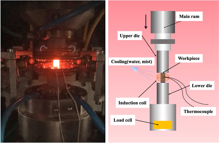
A view of the experiment (left) and a schematic illustration of the high-speed compression test machine (right). (Online version in color.)
The temperature is raised by electromagnetic induction heating with a high frequency of ±50 kHz. With the induction heating system, the temperature can be controlled precisely, and the heating time is short. To maintain a constant temperature, a PID feedback system is used in temperature control to compensate for the transient change of temperature in a very short time. The temperature is measured by attaching an R-type thermocouple on the surface of the specimen, and it also can measure the temperature rise of the surface during deformation.
There are two types of tools in the machine. One is the upper die and the other is the lower die. The compression is accomplished with the upper die, and the lower die is used to change the bottom dead of the compression position, which is useful in the high-speed double compression test. Both dies were made of silicon nitride (Si3N4). The material has a high elastic modulus E and low density ρ. A high ratio of them (
In the setup of the experiment, mica is inserted between the specimen and tool to minimize friction and the heat transfer effect. The material used in the experiment is JIS-S20C, which is a 0.2% low-carbon steel alloy. Its chemical composition is shown in Table 1.
| JIS-S20C (wt%) | ||||||||
|---|---|---|---|---|---|---|---|---|
| C | Si | Mn | P | S | Cu | Cr | Ni | Fe |
| 0.2 | 0.2 | 0.42 | 0.02 | 0.023 | 0.1 | 0.1 | 0.1 | Bal. |
The specimen is cylindrical with 12 mm height and 8 mm diameter. The specimen is compressed up to a reduction in height of 75%. The applied high strain rates are 10, 50, 100, 150, and 200 s−1, respectively. To avoid the mixed-phase effect, the compression is conducted at elevated temperatures of 900, 1000, 1100, and 1200°C, where the ferrite phase of 0.2% carbon steel is completely transformed to the austenite phase. Before compression, the specimen is heated to the target temperature at a heating rate of 10°C·s−1 and held for 180 s to ensure the complete austenite transformation, uniformly distribute the temperature inside the specimen, eliminate the internal strain, and homogenize the size of the equiaxed grains. The temperature history diagram is illustrated in Fig. 2.
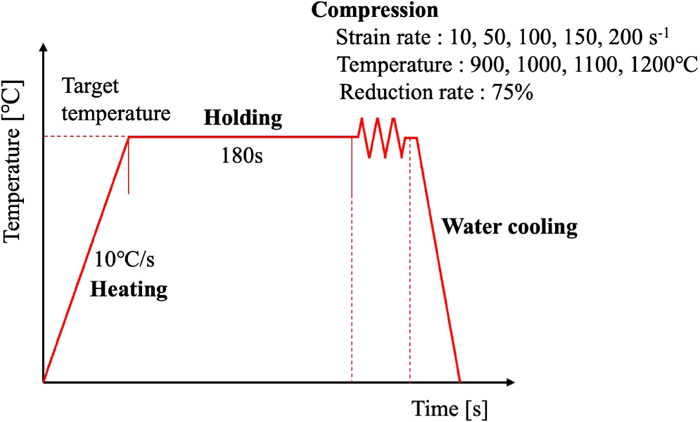
Experimental conditions, temperature history, and quenching method. (Online version in color.)
Maintaining a uniform high strain rate during deformation is highly challenging. If the strain rate and strain are 100 s−1 and 1, respectively, the total deformation time is around 0.01 s. Then, the response time of the machine is around 0.004 s, which cannot be ignored. Hence, each pattern data is extended to 0.004 s later to compensate for the effect. In addition, since a high strain rate is difficult to achieve from the start of compression, a run-up method accelerating the ram before compression is adopted.8)
Previously, the following equation is used to calculate stroke–time control pattern during deformation.10)
| (1) |
Here, h0 is the initial height of the specimen, and h is the instantaneous height of the ram during deformation. However, another problem arises due to the run-up method. The acceleration of the ram is yet to be solved and a new method to decelerate the ram is required. Otherwise, the axial strain rate increases sharply, which can affect the accuracy of the experimental flow curve.
The deceleration process is done by the following process.
(i) A pattern is made to obtain the result (i,1), and a new pattern is made that the time difference (Δt(i,1)) between the result (i,1) and the pattern (i,1) is the same as the time difference (Δt(i,2)) between the pattern (i,2) and the pattern (i,1).
(ii) After obtaining the result (i,2), the pattern (i,3) is made that the time difference (Δt(i,3)) between the pattern (i,3) and the pattern (i,1) is equivalent to the time difference (Δt(i,4)) between the result (i,2) and the pattern (i,3).
(iii) The result (i,3) is obtained and repeat the whole procedure until convergence to obtain the result (n,3).
As the initial pattern, stroke – time pattern using Eq. (1) is used. The schematic illustration of the deceleration method and strain rate control result is compared with that of the previous result in Fig. 3.10) At a strain rate of 50 s−1, the ram speed is properly controlled without the deceleration method. However, over 100 s−1, the deceleration method is shown to be effective.
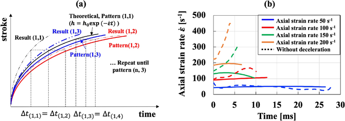
(a) A schematic illustration of the deceleration control method for the high-strain-rate compression test, and (b) the axial strain rate result comparison at the temperature of 1000°C between the previous method,10) and the deceleration method. (Online version in color.)
At high strain rates, oscillation due to the elastic response of the test machine occurs. The Savitzky–Golay filtering technique is used to increase precision without greatly distorting the entire tendency. The stress affected by the vibration investigated in our previous research10) is described as
| (2) |
| (3) |
Axial stress-strain relationships can be determined by compensating bulge deformation by the method of Suzuki et al.,13) but a uniaxial flow curve will be obtained by the inverse analysis of compressive force–stroke data obtained experimentally.11) The correction of stroke, which is the compensation of change in the mica thickness and deflection of the test machine, was also taken into the account. The vibration-compensated apparent stress–axial strain curve result at 1000°C is presented in Fig. 4.
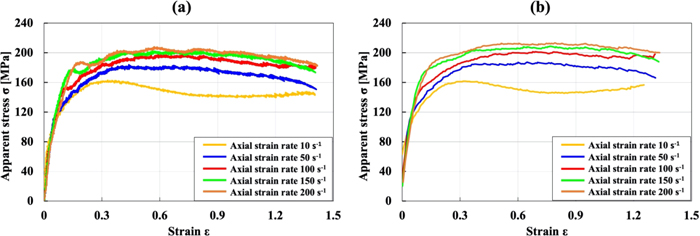
Apparent stress–axial strain curve at the temperature of 1000°C (a) before filtering, and (b) after filtering out vibration patterns. (Online version in color.)
The constitutive equation for the flow curve used in the inverse analysis is presented by Yanagida et al.,11) where the softening phenomenon during deformation was taken into the account. The equation is formulated as
| (4) |
| (5) |
In Eq. (4), F1 (plastic modulus), n (work hardening exponent), εc (critical strain), and F3 (steady-state stress) are independent parameters that can be obtained by inverse analysis, and all of them are material constants that have clear individual physical meanings. To obtain the generalized flow stress σf in Eq. (5), strain rate and the strain rate sensitivity m0 are considered. As the initial value of the sensitivity, m0 = (1.6×10⁻⁴)T − 0.1031 is applied,12) where T is the deforming temperature.
3.2. Internal Temperature DistributionThe distributed internal temperature is obtained using thermal FEA by inverse analysis, and it is calculated using the following equations.
| (6) |
| (7) |
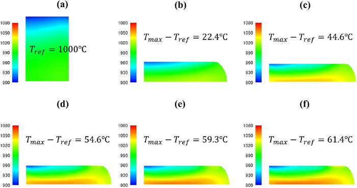
Internal temperature distribution at 1000°C (a) before compression, and at the strain rates of (b) 10, (c) 50, (d) 100, (e) 150, and (f) 200 s−1. (Online version in color.)
Figure 5 shows that the temperature is higher in the center of the specimen and lower near the surface. The difference becomes larger when the strain rate increases. The maximum temperature in the center reaches approximately 1061°C when the strain rate is 200 s−1, whereas it reaches only 1022.4°C at the strain rate of 10 s−1. In other words, it can be concluded that the specimen is deformed unevenly at high strain rates. The flow stress
| (8) |
By using
| (9) |
The initial temperature sensitivity A0 is chosen to be 4260.12) Also,
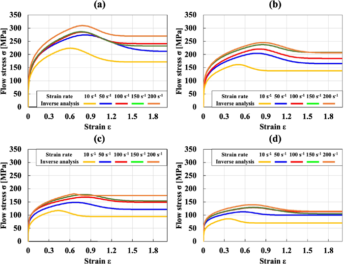
Flow curves obtained by inverse analysis at temperatures of (a) 900, (b) 1000, (c) 1100, and (d) 1200°C. (Online version in color.)
Figure 7 illustrates that the flow stress obtained the inverse analysis is greater than the experimental one because of the internal heat generation. During the calculation, an increased temperature is reflected for both of the calculated load and the experimental load. After the calculation using inverse analysis, each optimized independent parameter is obtained. When the reference temperature is applied to the constitutive equation as illustrated in Fig. 7(b), the flow stress increases, and the difference in Figs. 4 and 6(b) shows that it corresponds to the theory.
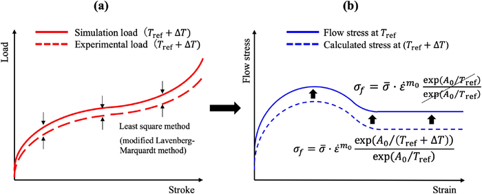
Schematic illustrations of (a) the inverse analysis calculation using temperature-increase-reflected load data and (b) the flow stress increase after applying the reference temperature. (Online version in color.)
As shown in the result of inverse analysis in Fig. 6, the flow curves at high strain rates are not arranged in an orderly manner and show greater errors. Therefore, a regression method is required to determine their correct relationship and to obtain the regressed flow stress σ*. All independent parameters F1, εc, n, and F3 and initial sensitivities m0 and A0 should be altered to F1*, εc*, n, F3*, m, and A, respectively.12)
For each condition, the critical strain εc, the point indicating the starting point of the dynamic recrystallization varies and is fitted by the following equation.
| (10) |
By optimizing the fitting, the constants a, b, and c are determined to be 0.096, 0.197, and 5441.153, respectively. The fitting result and the data points are shown in Fig. 8. The critical strain from the inverse analysis generally increases at a strain rate lower than 100 s−1, but it does not seem to be sensitive to strain rate higher than 100 s−1. There is controversy over the relationship of critical strain with the strain rate. Senuma et al. argued that critical strain is independent of strain rate.1) Recently, there are more research results showing a proportional relationship of critical strain with strain rate.16)
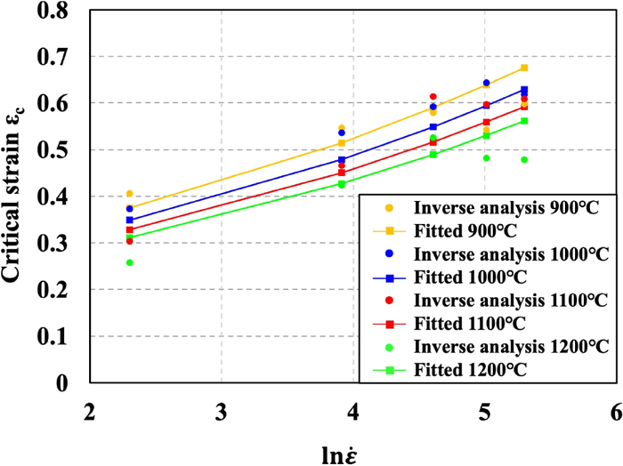
Regression of critical strain εc obtained by inverse analysis. (Online version in color.)
By considering the function continuity at critical strain, the dependent parameters F2, εmax, and a are changed to F2*, εmax*, and a*, respectively, using the regressed independent parameters F1*, εc*, n, and F3*.
All determined parameters are listed in Table 2.
| Independent parameters | F1* | n | F3* |
| 123.6 | 0.212 | 94.64 | |
| Strain rate sensitivity m | m = (−2.8×10⁻⁷ )∙T2+0.00092∙T−0.614 | ||
| Reference temperature T* | 1323 K | ||
| Temperature sensitivity A | 5628.5 | ||
| Critical strain εc* | |||
Using them, the complete formulation of the generalized flow curve is expressed as
| (11) |
The generalized flow curves of 0.2% carbon steel at high strain rates from 10 to 200 s−1, and flow curves obtained by the inverse analysis in Fig. 6 are shown in Fig. 9 again.
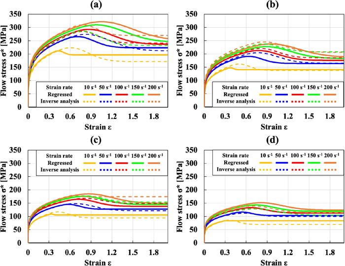
Regressed flow curves at temperatures of (a) 900, (b) 1000, (c) 1100, and (d) 1200°C. (Online version in color.)
The result shows that an abrupt drop after peak stress in the flow curve is apparent. Jonas et al. obtained a flow curve at high strain rates by the extrapolation method and showed that the flow curve at a high strain rate is a DRX-type flow curve.17) They assumed that the higher the strain rate, the larger the DRX volume fraction. There have been several research results demonstrating that a high strain rate can produce an abundance of the twinning structure during deformation. Mandal et al. argued that such a twinning structure in the grain occurring because of the high strain rate can be an additional nucleation site for DRX.18) However, Yanagida et al. found that although the flow curve is a typical abruptly dropping DRX type, the actual DRX rate can be very low.19)
4.2. Comparison with the Regressed Flow Curve at Intermediate Strain RatesThe complete form of the flow curve equation is described as follows at strain rates of 50 to 200 s−1.
| (12) |
| (13) |
| (14) |
Dependent parameters F2*, a*, and εmax* are obtained by applying the law of continuity at the regressed critical strain εc*. Their formulations are described as
| (15) |
| (16) |
| (17) |
The generalized flow curve, which is regressed using the result obtained at the intermediate strain rates of 1, 10, and 50 s−1, was obtained by Yanagida et al.12) It can be used to calculate the flow curves at strain rates of 50, 100, 150, and 200 s−1 at 1000°C. Flow curves extrapolated from a previous equation12) are shown with the newly regressed flow curves at the high strain rates in the current investigation in Fig. 10.
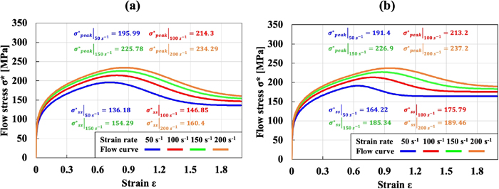
(a) Extrapolated flow curve regressed from an intermediate strain rate and (b) flow curve at high strain rates obtained in the current investigation. (Online version in color.)
The overall peak stress level for the two results is not so different, but the steady-state stress for the extrapolated curve is lower than the flow curve obtained in the current investigation. Also, critical strain in the current investigation is 0.05 higher than that obtained from the extrapolated curve. Temperature sensitivity A obtained from the above result is 5628, whereas that obtained in the previous research is 4260. The stress difference between the extrapolated flow curve and flow curve obtained in the current research is revealed using inverse analysis by reflecting significant temperature rises during deformation at the high strain rate, as mentioned in Section 3.2. The main reason for the difference can be the metallurgical phenomenon resulting from the high strain rate deformation.
Microstructure observation is conducted by EBSD equipped with a field-emission scanning electron microscope (FE-SEM, JEOL 7100 F) to demonstrate the effect of deformation rate on the flow curve at high strain rates range. Since 0.2% carbon steel alloy transforms from austenite at elevated temperature to ferrite pearlite martensite structure after cooling, SUS316 austenitic stainless steel is used instead for the EBSD analysis of microstructure. The deformed specimen is cut in half with a fine cutter in the compression direction, hot-mounted, and polished using OP-U non-drying colloidal silica suspensions. The scanned results microstructure deformed by two different strain rates 50 s−1 and 200 s−1 are compared in Fig. 11. The initial temperature is 1000°C.
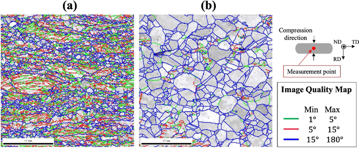
Image quality maps obtained by EBSD using SUS316 austenitic stainless steel at initial temperature of 1000°C, 75% reduction rate of height, and strain rates of (a) 50, and (b) 200 s−1. (Online version in color.)
It shows that deformation twinning is apparent at the high strain rate of 200 s−1, whereas it is less at 50 s−1. It is acknowledged that twinning can lead to an increase in the work hardening rate during the deformation of face-centered cubic (FCC) metals and alloys with the low stacking fault energy (SFE).20) Elevated temperatures due to plastic work at a higher strain rates, or the higher deformation rate itself, leads to an increase in grain boundary migration, which eventually can accelerate deformation twinning.21) In addition, grain size is much smaller in the deformed specimen at a lower strain rate, although DRX grain size is smaller at higher strain rate. The above results would be the examples to claim the necessity of high-speed deformation tests to identify the flow curve by using the inverse analysis, although steel chemistry is completely different between S20C and SUS316. In addition, grain size is much smaller in the deformed specimen at lower strain rate in this experiment of SUS316, but the dynamically recrystallized grain size is smaller at higher strain rate in plain carbon steels.1) A simple extrapolation cannot reflect the difference in flow stress in Fig. 10 due to the possible twinning effect for example. As a result, it can be concluded that the extrapolation from the generalized flow curve regressed using intermediate strain rate data is different from the directly obtained result by the high-speed compression test.
The flow curve of 0.2% carbon steel at high temperature and high strain rate was studied.
(1) Deceleration of speed of ram is realized using a specialized control method for Thermecmastor-Z 15 ton machine to obtain a uniform axial strain rate.
(2) A vibration filtering method that takes into consideration the elastic response of the compression test machine at a high strain rate for the frequency of 1000 Hz was used to eliminate the effect. A Savitzky–Golay filtering method was chosen as a numerical method of effectively smoothing the oscillating data.
(3) By the inverse analysis method, the flow curve was obtained. The compensation of the internal heat generation and the highly distributed temperature, which leads to inhomogeneous deformation, were the main reason why the apparent stress–axial strain curve greatly differed from the calculated result.
(4) A regression of the independent parameters and the sensitivity of the strain rate and temperature was done to obtain the generalized flow curve that can include a wide range of strain rates, strains, and temperatures.
(5) A flow curve regressed from intermediate strain rate data was extrapolated to high strain rates, and it was compared with the regressed flow curve obtained in the current investigation. The steady-state stress of the extrapolated flow curve greatly differed from the directly obtained result. The difference may have been caused by the twinning effect due to high-strain-rate deformation. It can be concluded that the extrapolation method from low and intermediate strain rates to high strain rates is inappropriate.