A Modified Random Sampling Method Using Unidirectionally Solidified Specimen: Solute Partition Coefficients in Fe–Cr–Ni–Mo–Cu Alloys

Abstract

A random sampling method using Fe-19.9 mass% Cr-24.8 mass% Ni-4.5 mass% Mo-1.5 mass% Cu alloy quenched during unidirectional solidification was applied to examine the measurement accuracy of the solute partition coefficients between the solid and liquid phases. Better agreement between the solute profiles obtained by the random sampling and Scheil’s equation was observed at appropriate regions where the solid fraction ranged from 0.9 to 1 at quenching. The partition coefficients of Cr, Ni, Mo, and Cu were determined to be 0.95, 1.01, 0.71, and 0.84, respectively. The values obtained using the present method agreed well with the values measured using the in-situ measurement method, which is recognized to be a reliable technique. The developed technique, which uses conventional equipment and techniques such as a unidirectional solidification furnace and scanning electron microscopy/energy-dispersive X-ray spectroscopy, requires less time to determine the solute partition coefficients than conventionally used techniques. Thus, the modified random sampling method presented in this study can be used for systematic measurements of solute partition coefficients.

1. Introduction

Common austenitic stainless steels such as SUS304 and SUS316 do not have sufficient corrosion resistance for use in severe environments such as seawater, hydrochloric acid, and sulfuric acid.^1,2) Fe–Cr–Ni–Mo–Cu stainless steels were developed to improve the corrosion resistance of common austenitic steels by increasing the Cr and Ni contents and adding Mo and Cu.^1,2,3) Increasing the Ni content not only stabilizes the austenite phase but also improves the general corrosion and stress-corrosion-cracking resistances.³⁾ The Mo addition improves the pitting corrosion resistance, and the Cu addition improves the corrosion resistance in a sulfuric acid environment.^1,3) Thus, Fe–Cr–Ni–Mo–Cu stainless steels have been used for various applications, for which high corrosion resistance is required. These include in marine structures, chemical plants, and desulfurization equipment for coal power plants.

Microsegregation formed in the interdendritic region is commonly observed in the as-cast microstructure and can degrade the material properties, including the hot workability, weldability,^4,5,6) and corrosion resistance.⁷⁾ Therefore, prediction of the microsegregation level in the as-cast microstructure is valuable to achieve the required corrosion resistance. However, prediction of the microsegregation profile in as-cast ingots remains difficult because the solute partition coefficients have not yet been systematically measured for multicomponent alloys. There are uncertainties in the partition coefficients as a function of the liquid composition along the solidification path, especially for high-concentration alloys such as Fe–Cr–Ni–Mo–Cu alloys. Therefore, it is of interest to develop a time-saving and reliable technique that uses conventional apparatuses.

Several methods have been developed to determine the partition coefficients. In the conventional method^8,9,10) (referred to as the quenching method), equilibrium between the solid and liquid phases is achieved by holding a specimen at a temperature between the solidus and liquidus temperatures followed by quenching of the specimen. The chemical compositions of the solid and liquid regions before quenching are measured using chemical analysis, either scanning electron microscopy/wavelength-dispersive X-ray spectroscopy (SEM/WDX) or SEM/energy-dispersive X-ray spectroscopy (EDS). The advantages of this method are 1) the high accuracy of the composition measurements, 2) the ability to measure dilute elements, and 3) the use of conventional apparatuses. However, the disadvantages are 1) the time required to reach equilibrium, 2) the difficulty of identifying the solid–liquid interface before quenching, and 3) the obtainment of a single measurement for each experiment.

Recently, an in-situ measurement method based on X-ray transmission imaging and X-ray fluorescence analysis using synchrotron radiation (referred to as the in-situ method) was developed^11,12) to determine the partition coefficients with high accuracy. In a previous report,¹²⁾ the partition coefficients for a Fe-19.9 mass% Cr-24.8 mass% Ni-4.5 mass% Mo-1.5 mass% Cu alloy at the beginning of solidification were determined to be 0.96, 0.97, 0.70, and 0.86 for Cr, Ni, Mo, and Cu, respectively. The technique is considered to have high measurement accuracy because the X-ray fluorescence spectra from the liquid and solid phases near the solid–liquid interface are measured in situ. The in-situ measurements during the unidirectional solidification keeping the flat interface allow the partition coefficients to be tracked along the solidification path. The solute partition coefficients for 56 compositions were measured in the study,¹²⁾ demonstrating the potential of this in-situ technique for systematic measurements. However, this technique has certain limitations. One is that light elements such as Al, Si, Mg, S, and P cannot be measured using the current apparatus because the fluorescence X-rays with lower energies are absorbed by the windows of the specimen holder and the vacuum chamber. The other limitation is the limited access to synchrotron radiation facilities. Thus, the development of a complementary method is expected to strengthen the advantages of the in-situ measurement method.

A random sampling method^{10,13,14,15,16)} has also been used to determine the partition coefficients for various alloys. In this method, SEM/EDS measurements of the solidification structure are performed at 100 or more points on a grid. If an appropriate grid is selected, the measured compositions are expected to represent the microsegregation. The compositions are sorted to obtain the solute profiles of the microsegregation, and the partition coefficients are determined by analyzing the profiles. The solute partition coefficients in a Fe-19.9 mass% Cr-24.8 mass% Ni-4.5 mass% Mo-1.5 mass% Cu alloy determined using this method¹⁰⁾ were 0.95, 1.01, 0.78, and 0.88 for Cr, Ni, Mo, and Cu, respectively. The partition coefficients measured using the random sampling tended to shift toward 1 compared with those measured using the in-situ measurement method.¹²⁾ These tendencies could be caused by diffusion in the solid phase during/after solidification. Although the random sampling method is simple and timesaving, further improvement in the accuracy is required for accurate prediction of the microsegregation.

On the basis of this background, this study focuses on the fabrication of the solidification structure for the random sampling method. Unidirectional solidification has been widely used to clarify various solidification phenomena.^17,18,19) The dendritic structures from the dendrite tips to the root in constrained growth can be preserved by quenching the specimen during the unidirectional solidification. The results of the random sampling at various positions in the quenched specimen are compared with the partition coefficients measured using the in-situ measurement method.¹²⁾ The authors believe that the accuracy can be improved by controlling the solidification structure for the random sampling. Based on this validation, this study proposes a new measurement procedure for the random sampling method. Because the method allows the solute partition coefficients to be measured efficiently, the proposed procedure is expected to contribute to the building of a comprehensive database.

2. Experimental

2.1. Determination of Solid Fraction as a Function of Temperature

Table 1 shows the chemical composition of Fe–Cr–Ni–Mo–Cu alloy, which is equivalent to SUS 890L. Fully austenitic solidification mode was indicated by a thermodynamic calculation using Thermo Calc²⁰⁾ and experiments.¹⁰⁾ Pure Fe, Cr, Ni, Mo, and Cu were melted in a magnesia crucible using an induction furnace to produce an ingot. The ingot was forged followed by peeling of surface scale.

Table 1. Chemical compositions of the alloy (mass%).

Cr	Ni	Mo	Cu	Fe
19.89	24.82	4.50	1.47	bal.

Differential scanning calorimetry (DSC) was used to determine the solid fraction, f_S, in the unidirectionally solidified specimen (described in 2.2). A specimen with a diameter of 10 mm and a thickness of 0.36 mm was heated up to 1450°C and cooled at a cooling rate of 0.33 K/s. The cooling rate was almost equal to that in the unidirectional solidification experiment. In the cooling procedure of DSC, the heat release rate, q(t), due to the solidification was measured as a function of time, t. Here, the latent heat per mass unit was assumed to be constant during solidification. The solid fraction as a function of time is simply given by Eq. (1).   

$$f_s\left(t\right)={\int }_{t_s}^{t}q\left(t\right)dt/{\int }_{t_s}^{t_e}q\left(t\right)dt$$(1)

Here, t_s and t_e are the start time and the end time of solidification. Since temperature was also measured as a function of time in DSC, the solid fraction as a function of temperature was obtained.

2.2. Unidirectional Solidification

Figure 1 presents a schematic illustration of the unidirectional solidification apparatus, in which dendrites grow upward at a given withdrawing rate. A cylindrical specimen of 10 mm in diameter was prepared from the forged ingot. The specimen in an alumina tube with 11-mm inner diameter and 430-mm length was placed on a stage at the bottom of the furnace. The melted zone was 60 mm from the top before the specimen was withdrawn. The stage was withdrawn at a velocity of 5 mm/min (83 μm/s). After withdrawing 50 mm (600 s), the specimen was quenched in a water bath as shown in Fig. 1.

Fig. 1.

Unidirectional solidification apparatus. (Online version in color.)

2.3. Observation of Microstructure

The cross sections parallel to the withdrawing direction were polished and etched by 10 mass% aqueous oxalic acid solution with a current electrolytic density of 50 mA/cm² at room temperature. The dendritic structures on the sections were observed with an optical microscope, and the dendrite arm spacings were measured. The backscattered electron images of the cross sections perpendicular to the withdrawing direction were also observed at positions of 5, 15, 20, 25, 28, and 31 mm from the solid–liquid interface before withdrawing. The cross sections were used for analysis using the random sampling method.

2.4. Random Sampling Method

The observation area for the random sampling was 1 mm in width and 0.7 mm in height. EDS analyses were performed accounting for the previous gridding ideas;^13,15) the measurement points are taken more than 100 points as square-meshes that are larger than secondary arm spacing. Therefore, 300 points were taken on a grid with intervals of 80 μm which was larger than the secondary arm spacing. In addition to the previous ideas, the width and height of the gridded analysis area were larger than the primary dendrite arm spacing of 250 μm.

The simple sorting method,^13,14) in which the solute concentrations are sorted independently, does not always satisfy the law of mass conservation. Thus, the procedure causes a slope segment,¹⁴⁾ which is an artificial deviation near the solid fraction f_S = 0; this deviation causes difficulties in the determinations. Thus, two sorting methods were proposed to improve the sorting accuracy: sorting of a major element (referred to as the Fe sort)²¹⁾ and WIRS¹⁶⁾ (weighted interval rank sort). The Fe sort rearranges the solute concentrations according to the ranking of Fe contents to maintain mass conservation at each point. WIRS rearranges the solute concentrations according to the weighted-average values of the solute concentrations. The weighted-average value is determined using all the solute concentrations.¹⁶⁾ The profiles obtained from the both methods were compared with each other to understand the difference attributed to the sorting methods.

3. Results and Discussion

3.1. Solid Fraction f_S as a Function of Temperature

Figure 2 shows the solid fraction measured by DSC as a function of temperature at a cooling rate of 0.33 K/s. Solidification began at 1398°C and was completed at 1355°C. The temperature of 1398°C agrees with the liquidus temperature measured in a previous study.¹⁰⁾ The relationship between the solid fraction and temperature was used to estimate the solid fraction distribution in the unidirectionally solidified specimen at quenching.

Fig. 2.

Evolution of solid fraction f_S with temperature determined using DSC at a cooling rate of 0.33 K/s.

3.2. Microstructure in Quenched Specimen during Unidirectional Solidification

Figure 3 shows the microstructure parallel to the withdrawing direction. The position of the solid–liquid interface before withdrawing the specimen was designated to be zero, and thus, the vertical position corresponds to the solidification length. As shown in Fig. 3, the total solidification length was 32 mm, which was shorter than the withdrawn length of 50 mm. The average growth velocity, V, calculated from the solidification length and withdrawing duration, was 53 μm/s. As shown in Fig. 3, the primary dendrite arms tended to be nearly in the withdrawing direction. The typical microstructure observed in unidirectionally solidified specimens was obtained.

Fig. 3.

Optical microscope images of microstructure parallel to the withdrawing direction. (Online version in color.)

Figure 4 shows close-up views of the dendritic structures at 5, 15, 20, 25, 28, and 31 mm from the solid–liquid interface before withdrawing. The averaged secondary arm spacing, λ₂, was 69 μm at 25 mm. The cooling rate, R, was calculated to be 0.33 K/s using the following relation:¹⁰⁾   

$${\lambda }_2=43.6R^{-0.41}.$$(2)

Fig. 4.

Close-up views of 5, 15, 20, 25, 28, and 31 mm positions from the position of the solid–liquid interface before withdrawing. (Online version in color.)

Thus, the temperature gradient, G, at 25 mm was estimated to be 0.006 K/μm by assuming the relationship G = R/V. The temperature at the tip position of dendrites is assumed to be the liquidus temperature of 1398°C. The estimated temperatures and solid fraction at each position just before quenching are also indicated in Figs. 3 and 4.

Backscattered electron (BSE) images of the dendritic structures perpendicular to the withdrawing direction are presented in Fig. 5. The brightness in the images reflects the segregation of Mo element. The contrast induced by the microsegregation was relatively blurred at 5, 15, and 20 mm, where the solidification was completed before quenching. The blurred images suggest that the solid diffusion reduced the microsegregation. The microsegregation between the dendrite arms was clearly observed at 25 and 28 mm, where the solid fraction ranged from 0.9 to 1.0 at quenching. The fine dendritic structure produced by quenching was observed at 31 mm, and the microsegregation induced by the rapid growth was clearly observed.

Fig. 5.

Back-scattered electron images of the dendritic structures perpendicular to the withdrawing direction.

3.3. Solute Profiles Obtained by Random Sampling

Figures 6(a) and 6(b) show (C_S/C₀), the concentrations in the solid (C_S) normalized by the average concentration (C₀) for Mo, in the sequence of measurements and a profile rearranged by the Fe sort, respectively. Although a variation of ± 0.1 was observed in the Fe-sort profile, the concentration increased with increasing solid fraction. In addition, the slope segment mentioned in 2.4 was not observed in the rearranged profiles.

Fig. 6.

Example of random sampling method at 5-mm position: (a) EDS multipoint analysis result for Mo and (b) concentration profile of Mo obtained by Fe sort.

The solute profiles of the Cr, Ni, Mo, and Cu elements, which were sorted by the Fe sort, are presented in Fig. 7. The profiles at different positions indicated by colors were plotted in the figure. The profiles of Cr, Mo, and Cu increased with increasing solid fraction, whereas that of Ni decreased. Figure 8 shows the profiles sorted by the WIRS. The variation in the Mo profile sorted by the WIRS was slightly smaller than that sorted by the Fe sort. In the WIRS, the weighted compositional value of Fe was larger than that of the other elements. Thus, the profiles obtained using the two sorting methods were similar.

Fig. 7.

Concentration profiles of the solute elements rearranged by Fe sort.

Fig. 8.

Concentration profiles of the solute elements rearranged by WIRS.

The concentration of Cr slightly increased with increasing solid fraction. The concentrations were in good agreement with each other for fs < 0.8, and the concentrations at the positions of 25 and 28 mm were slightly larger in the range of 0.8 < fs < 0.98. The concentrations at 25, 28, and 31 mm rapidly increased for fs > 0.98 and were as high as 1.4.

The concentration of Ni was nearly 1 for fs < 0.98, indicating that the partition coefficient was nearly 1. In the Ni profiles, the profiles at the different positions were similar, and no differences were observed except for the deviations at fs=1 at 25, 28, and 31 mm. The deviation was caused not by the solute partition but by the formation of the σ-phase at the end of solidification.²²⁾ Thus, the appearance of the rapid increases/decreases only at the final stage indicated that the sorting was valid. In addition, the rapid increases/decreases at 25, 28, and 31 mm indicate that the concentration profiles depend on the position in the unidirectionally solidified specimen.

The concentration profiles of Mo at 25 and 28 mm were higher than those at 5, 15, 20, and 31 mm for fs > 0.85. This tendency is the same as that observed in the concentration profiles of Cr. Although the sorted concentrations of Cu were scattered because of the low initial concentration of 1.5 mass% Cu, the concentrations increased with increasing solid fraction.

Summarizing above, the tendencies indicate that Cr, Mo and Cu atoms are partitioned to the liquid phase while Ni atoms are slightly partitioned to the solid phase at the solid–liquid interface.

3.4. Fitting to Scheil’s Model

In the random sampling method, a model that analyzes the solute profile (obtained by sorting) is needed to determine the solute partition coefficient. Scheil’s equation²³⁾ is one of the well-known models to predict the microsegregation. The model assumes no solute diffusion in the solid phase and perfect mixing in the residual liquid phase. The determination of the partition coefficients based on Scheil’s equation is advantageous because the assumptions in the model are well defined and the fitting to the equation is simple. However, it is rather difficult to determine the effect of solid diffusion on the microsegregation in the solidification structure.

In the specimen quenched during unidirectional solidification, the solute profiles depended on the sample positions, as shown in Figs. 7 and 8. The solid diffusion before quenching and the rapid solidification in the residual liquid phase by quenching can induce the deviation from Scheil’s equation. The sorted profiles are fitted to Scheil’s equation given by Eq. (3).   

$$\tilde{C}\left(f_s\right)=\frac{C_S}{C_0}=k{\left(1-f_s\right)}^{\left(k-1\right)}$$(3)

Here, the concentrations in the solid, C_S, are normalized by the average concentration, C₀. The partition coefficient, k, as a fitting parameter is determined by minimizing S (variance) given by Eq. (4).   

$$S={\displaystyle \sum }_{i=1}^N{\left[{\left(\frac{C_S}{C_0}\right)}^{\left(i\right)}-\tilde{C}\left(f_s^{\left(i\right)}\right)\right]}^2/N$$(4)

(C_S/C₀)⁽ⁱ⁾ is the normalized concentration of the i-th point in the sorted profile, and N the total number of random sampling points. The concentrations for f_S > 0.98 were not used for the fitting because of the σ-phase formation.

The k and S values at different positions are summarized in Table 2. The S values as a function of the positions are presented in Fig. 9. The S values of Mo and Cu show a minimum around the positions of 25 and 28 mm, where the solid fraction at quenching ranges from 0.9 to 1. However, the S values of Cr and Ni, of which the partition coefficients are nearly 1, did not depend on the position. As a result, the best fittings including all solute elements were obtained by the random sampling at positions ranging from 0.9 to 1 at quenching during the unidirectional solidification. In addition, the fitting results did not depend on the sorting methods in this study. Therefore, the results are discussed based on the Fe-sort data hereinafter.

Table 2. Partition coefficient k and S value of each solute at each position.

(a) Fe sort

Position (mm)	Moment of quench		Partition coefficient, k (–)				Variance, S (–)
	Temperature (°C)	Solid fraction from DSC, fS (–)	Cr	Ni	Mo	Cu	Cr	Ni	Mo	Cu
5	1226	1.00	0.97	1.01	0.82	0.91	0.00021	0.00015	0.00562	0.02918
15	1290	1.00	0.96	1.01	0.79	0.90	0.00019	0.00016	0.00407	0.02620
20	1321	1.00	0.96	1.01	0.79	0.90	0.00019	0.00015	0.00375	0.02466
25	1353	1.00	0.96	1.01	0.72	0.84	0.00020	0.00018	0.00295	0.02535
28	1372	0.92	0.95	1.01	0.70	0.84	0.00021	0.00018	0.00347	0.02394
31	1392	0.15	0.96	1.01	0.76	0.87	0.00021	0.00020	0.00560	0.02937

(b) WIRS

Position (mm)	Moment of quench		Partition coefficient, k (–)				Variance, S (–)
	Temperature (°C)	Solid fraction from DSC, fS (–)	Cr	Ni	Mo	Cu	Cr	Ni	Mo	Cu
5	1226	1.00	0.97	1.01	0.82	0.91	0.00018	0.00012	0.00471	0.02938
15	1290	1.00	0.96	1.01	0.79	0.90	0.00018	0.00013	0.00329	0.02561
20	1321	1.00	0.96	1.01	0.79	0.90	0.00017	0.00013	0.00270	0.02429
25	1353	1.00	0.96	1.01	0.72	0.85	0.00016	0.00019	0.00197	0.02508
28	1372	0.92	0.95	1.01	0.70	0.84	0.00014	0.00016	0.00292	0.02358
31	1392	0.15	0.96	1.01	0.76	0.86	0.00019	0.00015	0.00371	0.02929

Fig. 9.

Variation of S value with positions in the unidirectionally solidified alloy.

3.5. Validity of Solute Partition Coefficients

It is of interest to verify the validity of the partition coefficients determined in this study. Figure 10(a) shows the partition coefficients given by the best fitting as a function of the positions. The given values are also listed in Table 3. For the validation, the partition coefficients determined by the in-situ measurements¹²⁾ are presented in Fig. 10(b). The reported values obtained using the random sampling method in the previous study¹⁰⁾ and the quenching method¹⁰⁾ are also shown in Fig. 10(c). In the in-situ measurement method,¹²⁾ the compositions of the solid and liquid phases near the solid–liquid interface were measured in situ at 56 different compositions, and the partition coefficients of the solute elements were consistently given by regression functions within an error of ±10%. Thus, the partition coefficients determined by the in-situ measurement method¹²⁾ were used as the standard reference data. As shown in Fig. 10(b), the partition coefficients obtained by the in-situ measurement method¹²⁾ were 0.98 (Cr), 0.95 (Ni), 0.67 (Mo), and 0.84 (Cu). The previous study¹²⁾ noted that some discrepancies in the partition coefficients obtained using the in-situ measurement method¹²⁾ and the conventional random sampling method¹⁰⁾ were observed, as shown in Figs. 10(b) and 10(c).

Fig. 10.

(a) Partition coefficients k determined in this study compared with the values previously obtained using (b) the in-situ measurement method,¹²⁾ k_I, and (c) the quenching method, k_E, and random sampling method, k_R.¹⁰⁾

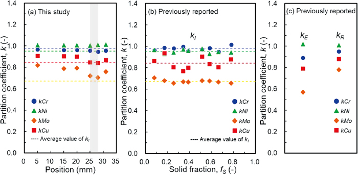
Table 3. Partition coefficient k determined in this study compared with previously reported values.

Method	Partition coefficient		Cr	Ni	Mo	Cu	Reference
Random sampling (unidirectionally solidified alloy)		k	0.95	1.01	0.71	0.84	This study
In-situ measurement (X-ray transmission imaging and X-ray fluorescence spectroscopy)	fS$\{\begin{array}{l}\\ \\ \\ \\ \\ \\ \\ \\ \\ \\ \\ \\ \\ \\ \end{array}$	kI					Kobayashi et al.12)
		0.08	0.96	0.97	0.70	0.86
		0.17	0.99	0.93	0.68	0.93
		0.26	0.98	0.94	0.66	0.80
		0.34	1.00	0.97	0.67	0.77
		0.39	0.96	0.96	0.67	0.80
		0.52	0.97	0.98	0.68	0.91
		0.58	0.98	0.93	0.68	0.83
		0.66	0.95	0.95	0.67	0.81
		0.78	1.02	0.94	0.65	0.88
		Ave.	0.98	0.95	0.67	0.84
Random sampling (ingot sample in a crucible)		kR	0.95	1.01	0.78	0.88	Yamamoto et al.10)
Conventional (isothermal holding at semi-solid state)		kE	0.89	1.02	0.57	0.79

The partition coefficients were determined at the positions of 25 and 28 mm, where the sorted profiles of Mo and Cu elements were well fitted by Scheil’s equation, 0.95 (Cr), 1.01 (Ni), 0.71 (Mo), and 0.84 (Cu). The partition coefficients obtained in this study were consistent with the values obtained using the in-situ measurement method.¹²⁾ The discrepancies were −3% (Cr), 6% (Ni), 6% (Mo), and 0% (Cu). The agreement within an error of ±6% proves that the random sampling method was improved using the specimen quenched during the unidirectional solidification.

3.6. Advantage of Random Sampling Method Using Unidirectional Solidification

The random sampling method using the solidification structure quenched in the range of 0.9 < fs < 1.0 during the unidirectional solidification yielded reliable partition coefficients. In other words, the sorted profiles in this solid fraction range were reproduced by Scheil’s equation. The conditions required for obtaining appropriate partition coefficients using the random sampling method are discussed in this section.

Figure 11 presents a schematic illustration of the solute concentration profiles in which (a) and (b) show the profiles before and during quenching, respectively. In the low-solid-fraction region indicated by line A–A’, the width of the liquid phase between the primary arms was nearly equal to the primary dendrite arm spacing, 250 μm measured from the structures shown in Figs. 3 and 4. The concentration profiles in the interdendritic region during the unidirectional solidification are presented in (a) of Fig. 11. The concentration reached a minimum between the primary arms; however, the concentration change was not large. If the solidification took even several seconds when the specimen was quenched, the growth velocity, V, in the interdendritic region was on the order of 10⁻⁴ m/s. The diffusion-layer thickness, which is defined by D/V, should be on the order of 10⁻⁵ m. Here, the diffusion coefficient, D, in the liquid phase is assumed to be 10⁻⁹ m²/s.²⁴⁾ Therefore, when the solid fraction is low, the formation of a solute built-up layer causes the solute profiles to deviate from Scheil’s model, as can be understood in (b) of Fig. 11. In addition, the fine dendrites produced by quenching cause some difficulties in the random sampling because the microsegregation domain size can be as small as the region affected by the beam for EDS measurements. Thus, it is obvious that the solidification structure in the low-solid-fraction region before quenching is not suitable for the random sampling method. In contrast, the width of the liquid phase between the primary dendrite arms before quenching is less than 20 μm in the high-solid-fraction region (0.9 < f_S < 1.0), indicated by B–B’. The diffusion coefficients in the solid and liquid phases are assumed to be on the order of 10⁻¹³ m²/s and 10⁻⁹ m²/s, respectively.^24,25,26) The local solidification time, t, was approximately 600 s in the present set-up. The diffusion lengths, which are simply defined by $\sqrt{Dt}$, were approximately 1 mm in the liquid phase and 10 μm in the solid phase. This estimation indicates that the solute concentration in the liquid phase was uniform and that the effect of the diffusion in the solid phase on the solute profile was relatively small. In addition, the fine dendritic structure did not form by quenching in the narrow region between the primary dendrites, as schematically illustrated in (b) of Fig. 11 and Figs. 3 and 4. Thus, the solidification condition in the high-solid-fraction regions mostly satisfies the assumptions for Scheil’s model.

Fig. 11.

Schematic illustration of the solute concentration profiles (a) before and (b) during quenching.

The solute profile in the solidification structure was modified by the solid diffusion after solidification. Here, the effect of the solid diffusion on the concentration profile is considered when the initial profile is given by Scheil’s model. According to the time-evolution diffusion equation, the change rate of the solute concentration, C, at the beginning is roughly proportional to the term F given by the following equation:   

$$F=\frac{d^2\tilde{C}}{d{f}_S{\hspace{0.17em}}^2}=k\left(k-1\right)\left(k-2\right){\left(1-f_S\right)}^{\left(k-3\right)}.$$(5)

For the partition coefficient k = 0.71 (Mo) in the alloy, the values of the F term are 11 at f_S = 0.8, 52 at f_S = 0.9, and 10100 at f_S = 0.99. The change due to the solid diffusion rapidly increases when f_S > 0.9. Thus, the solute profile rapidly deviates from Scheil’s model. Quenching of the specimen immediately before the solidification completes is required to preserve the solute concentration profile during the solidification.

In the unidirectional solidification, the growth velocity and temperature gradient are not completely but sufficiently independent parameters. For example, the domain size of microsegregation, such as the dendrite primary arm spacing, is mainly controlled by the growth velocity. Once the growth velocity is determined, the local solidification time is modified by the temperature gradient. Thus, it is possible to achieve the solidification conditions required for Scheil’s model (complete mixing in the liquid and negligible solid diffusion). In the present study, the solidification conditions were satisfied in the high-solid-fraction regions and the partition coefficients were simply determined by applying Scheil’s model. It should be noted that the argument is valid not only for the Fe–Cr–Ni–Mo–Cu alloys but also for alloy systems consisting of substitutional elements. Because the present method uses conventional techniques such as unidirectional solidification and SEM/EDS, the proposed method can be extensively used to determine the solute partition coefficients for alloy systems containing substitutional elements.

The in-situ measurement^11,12) determines the partition coefficients of elements for which the fluorescence X-ray energies are higher than 5 keV with sufficient accuracy. However, there are several disadvantages of the in-situ measurement method. One is that fluorescence X-rays of light elements cannot be measured. The other is that access to synchrotron radiation facilities is limited. From an industrial viewpoint, it is valuable to extensively apply the random sampling method using the unidirectional solidification to measure the solute partition coefficients and to use the in-situ measurement method to ensure the reliability of the random sampling and to obtain reference data at the standard compositions.

4. Conclusions

An attempt was made to improve the accuracy of measuring the partition coefficient in Fe–Cr–Ni–Mo–Cu alloy using a modified random sampling method. In the method, the solidification structures were obtained by quenching the specimen during unidirectional solidification. The solute profiles were obtained at different growth positions using the random sampling method.

(1) The solute profiles at the positions where the solid fraction ranged from 0.9 to 1 at quenching were represented by Scheil’s equation.

(2) The solute partition coefficients determined in the solid fraction region were 0.95 (Cr), 1.01 (Ni), 0.71 (Mo), and 0.84 (Cu).

(3) The partition coefficients were consistent with the partition coefficients determined using the in-situ measurement method.¹²⁾ The discrepancy between the two methods was less than 10%.

(4) In the present set-up, in the region in which the solid fraction ranged from 0.9 to 1, the back-diffusion in the solid phase was negligible and the concentration between the dendrite arms was uniform. Quenching did not cause deviation from Scheil’s model. The required condition is expected to be satisfied generally because two different control parameters (the growth velocity and temperature gradient) were optimized in the unidirectional solidification.

(5) The proposed method can be widely used for alloy systems composed of substitutional elements with relatively low diffusion coefficients.

(6) The proposed method, which uses conventional apparatus without accessibility limitations, will contribute to the building of systematic datasets using comprehensive measurements.

Acknowledgments

The synchrotron radiation experiments were performed as a General Proposal for Industrial Application (2017B1581 and 2018A1586) at beamline BL20B2 at SPring-8 with approval of the Japan Synchrotron Radiation Research Institute (JASRI). The development of the in-situ measurement apparatus was supported by JSPS KAKENHI Grand Number JP17H06155.

References

• 1)   K.  Osozawa: Corros. Eng. (Jpn.), 27 (1978), 256 (in Japanese).
• 2)   M.  Yabe and  N.  Koide: Tetsu-to-Hagané, 99 (2013), 415 (in Japanese).
• 3)  Stainless Steels Handbook, eds. by R. Tanaka and Japan Stainless Steel Association, The Nikkan Kogyo Shimbun, Tokyo, (1995), 554 (in Japanese).
• 4)   A.  Yamanaka,  K.  Nakajima and  K.  Okamura: Ironmaking Steelmaking, 22 (1995), 508.
• 5)   T.  Maki: Tetsu-to-Hagané, 74 (1988), 1219 (in Japanese).
• 6)   J. A.  Brooks and  A. W.  Thompson: Int. Mater. Rev., 36 (1991), 16.
• 7)   K.  Saito: J. Jpn. Weld. Soc., 50 (1981), 251 (in Japanese).
• 8)   Z.  Morita,  T.  Tanaka,  N.  Imai,  A.  Kiyose and  Y.  Katayama: Trans. Iron Steel Inst. Jpn., 28 (1988), 198.
• 9)   T.  Tanaka,  N.  Imai and  Z.  Morita: Tetsu-to-Hagané, 75 (1989), 432 (in Japanese).
• 10)   K.  Yamamoto,  K.  Narikiyo,  N.  Sasaguri,  H.  Miyahara,  K.  Mizuno and  H.  Todoroki: Tetsu-to-Hagané, 103 (2017), 703.
• 11)   I.  Uwabe,  K.  Dobara,  K.  Morishita,  T.  Nagira and  H.  Yasuda: Tetsu-to-Hagané, 103 (2017), 678 (in Japanese).
• 12)   Y.  Kobayashi,  K.  Dobara,  H.  Todoroki,  C.  Nam,  K.  Morishita and  H.  Yasuda: ISIJ Int., 60 (2020), 276.
• 13)   M. N.  Gungor: Metall. Trans. A, 20 (1989), 2529.
• 14)   W.  Yang,  K.-M.  Chang,  W.  Chen,  S.  Mannan and  J.  DeBarbadillo: Metall. Mater. Trans. A, 31 (2000), 2569.
• 15)   W.  Yang,  W.  Chen,  K. M.  Chang,  S.  Manna and  J.  DeBarbadillo: Superalloys 2000, (Seven Springs), ed. by T. M. Pollock, R. D. Kissinger, R. R. Bowman, K. A. Green, M. McLean, S. Olson and J. J. Schirra, TMS, Pittsburgh, PA, (2000), 75.
• 16)   M.  Ganesan,  D.  Dye and  P. D.  Lee: Metall. Mater. Trans. A, 36 (2005), 2191.
• 17)   T.  Matsumiya,  H.  Kajioka,  S.  Mizoguchi,  Y.  Ueshima and  H.  Esaka: Trans. Iron Steel Inst. Jpn., 24 (1984), 873.
• 18)   Y.  Ueshima,  S.  Mizoguchi,  T.  Matsumiya and  H.  Kajioka: Metall. Trans. B, 17 (1986), 845.
• 19)   V. A.  Wills and  D. G.  McCartney: Mater. Sci. Eng. A, 145 (1991), 223.
• 20)   B.  Sundman,  B.  Jansson and  J.-O.  Andersson: Calphad, 9 (1985), 153.
• 21)   Y.  Kobayashi,  H.  Todoroki and  K.  Mizuno: ISIJ Int., 59 (2019), 277.
• 22)   E. O.  Hall and  S. H.  Algie: Metall. Rev., 11 (1966), 61.
• 23)   E.  Scheil: Z. Metallkd., 34 (1942), 70.
• 24)   Y.  Ono and  T.  Shigematsu: J. Jpn. Inst. Met., 41 (1977), 62 (in Japanese).
• 25)  Metals Data Book, eds. by Y. Waseda and The Japan Institute of Metals and Materials, Maruzen, Tokyo, (2004), 22 (in Japanese).
• 26)   A. F.  Smith and  G. B.  Gibbs: Met. Sci. J., 3 (1969), 93.