An Operator Behavior Model for Thermal Control of Blast Furnace

Abstract

To realize precise thermal control of a blast furnace, an operator model that imitates the behavior of skilled operators was developed using a convolutional neural network (CNN). Conventional thermal control systems suffer from large control errors when large disturbances occur, e.g., when low-quality materials are used. Despite these adverse conditions, capable operators are still able to take appropriate control actions by making the best use of sensor information. Such operators’ control actions were simulated by the CNN, and the validation results showed that the accuracy of the developed operator model was 71%. The operator model was then incorporated in the operation guidance system at actual furnaces. It was found that the operator model can cope with the severe situations where the material characteristics change or abnormal descent of the burden materials occurs.

1. Introduction

Low reducing agent ratio (RAR) has been pursued in the blast furnace operation for reducing the production cost and CO₂ emission. At the same time, high-quality raw materials are being depleted, and the use of low grade materials makes blast furnace operation even more difficult.¹⁾

Figure 1 shows the outline of blast furnace operation. The raw materials, i.e., coke and iron ore, are charged from the furnace top. While the solids descend through the furnace, they are heated by the ascending hot blast gas injected from the tuyeres around the furnace. As a result, the iron ore is eventually melted, forming liquid hot metal and its viscous byproduct, slag. The hot metal and slag are drained (i.e., tapped) from the tap holes at the bottom of the furnace.

Fig. 1.

Outline of blast furnace operation. (Online version in color.)

Precise temperature control of hot metal is crucial for realizing the efficient and stable operation. When the hot metal temperature (HMT) becomes too low, the temperature of the liquid slag is also low. This increases the viscosity of the slag, which makes it difficult to drain the slag smoothly from the furnace and decreases furnace productivity. On the other hand, an excessively high HMT must be avoided to prevent unnecessary consumption of the reducing agent.

Table 1 shows the classification of variables in this paper. To control HMT near the target value, the pulverized coal rate (PCR), i.e., amount of pulverized coal injected per unit of iron, is adjusted. The operators take control actions by predicting HMT in the near future from the trend of key process variables such as the top gas temperature (TGT) and the tuyere temperature, as shown in Fig. 1.

Table 1. Classification of variables in this work.

Variable	Unit
Key process variables (input variables of CNN)
Control error of HMT (ΔHMT)	°C
Coke ratio (CR), i.e., weight ratio of coke and iron	kg/t
Top gas temperature (TGT)	°C
Loading rate, i.e., frequency of raw material charging	ch./h
Tuyere temperature	°C
Manipulated variable
Pulverized coal ratio (PCR), i.e., pulverized coal per unit of iron	kg/t
Controlled variable
Hot metal temperature (HMT)	°C

Various thermal control systems have been developed to reduce the variance of furnace heat indices, e.g., HMT and the Si content of the hot metal. We developed a transient model-based operation guidance system and demonstrated its effect of reducing the control error of HMT in actual furnaces.^2,3) Radhakrishnan et al. applied a control system using a neural network model and stabilized the Si content.⁴⁾ The Si content has also been successfully controlled by a state-space model⁵⁾ or a support vector regression model.⁶⁾

Although these thermal control systems based on transient models^7,8) or statistical models^9,10) are practical under normal operating conditions, full-automatic control that can cope with abnormal conditions has not been reported. In particular, the transient models suffer from large prediction errors when material characteristics, e.g., reducibility of iron ore, fluctuate. The prediction accuracy of statistical models may deteriorate under unprecedented operating conditions. To realize full-automatic control, the control system must derive appropriate control actions even under the adverse conditions.

Capable operators can address such difficult situations by making the best use of the trend of key process variables. Since the control accuracy of a thermal control system is expected to improve by simulating such control actions of operators, we aimed at building a model that can simulate the control actions of skilled operators to maintain a constant HMT.

In the field of autonomous driving, a rapidly growing number of techniques are used to model the manual operation supported by experience and intuition. The driver’s models by convolutional neural network (CNN),¹¹⁾ hidden Markov model,¹²⁾ and inverse reinforcement learning¹³⁾ have been proposed. However, to the best of the authors’ knowledge, these techniques have not been applied in the steel industry. The operators at blast furnaces focus on the characteristic patterns in the transition of the key process variables and implement control actions. It is possible to simulate the operators’ decision-making in this manner by using CNN, because a CNN extracts characteristic patterns from images and performs prediction and classification based on the patterns.¹⁴⁾

The outline of this paper is as follows. The operator model using CNN is developed in Section 2. The accuracy of the operator model is validated by actual operation data in Section 3. The operator model is then incorporated into the conventional transient model-based operation guidance system, and its effect in reducing the variance of HMT is evaluated in Section 4. The conclusion is presented in Section 5.

2. Modelling Operators’ Control Actions

This section presents the method of modeling the operators’ control actions by CNN. The input and output variables of the CNN are defined, and the network architecture of the CNN is explained.

2.1. Input and Output of Operator Model

Table 1 summarizes the key process variables which have correlations with the thermal status of blast furnaces. These variables were determined through interviews with the operators. The trend of these variables is fed to the CNN. The loading rate is the number of burden material charges, i.e., a set of an iron ore layer and a coke layer, loaded from the furnace top per hour, and it indicates the descending speed of the materials. When the material descent is too fast, the iron ore is not fully reduced and HMT becomes too low. The tuyere temperature is the average of the temperatures measured by the thermocouples embedded in the 40 tuyeres around the furnace. Since the tuyere temperature is affected by the radiation from the coke bed and hot metal inside the furnace, it tends to change ahead of HMT, which is measured after the hot metal is tapped from the furnace.

Since the operators implement control actions so that HMT matches its target value, the deviation of HMT from the target value (ΔHMT) was entered into the CNN. For the other variables, there are no target values and the operators perform control actions in response to the trend of the variables. For this reason, the deviation from the mean value for the last 32 hours was entered into the CNN.

The output of the CNN is the operators’ control action. To control HMT, the pulverized coal ratio (PCR) [kg/t] is mainly used as the manipulated variable at the blast furnace. Figure 2 shows an example of the control action of increasing PCR. The origin of the horizontal axis is the moment when the control action was executed. The top five rows are the input variables of the CNN, and the bottom row shows PCR. The data period after the control action was performed, which is not fed to the CNN, is plotted by the dotted line in Fig. 2. Operators increased PCR at 0 h in response to the decrease of the tuyere temperature and TGT during the past 5 hours. As a result, they successfully suppressed the drop of HMT, and the target HMT was achieved at 10 h.

Fig. 2.

Example of control action of increasing PCR. (Online version in color.)

The operation amount of PCR is generally 5 kg/t in one control action, as shown in the bottom row of Fig. 2. Since the amount of one PCR control action normally does not vary, it is sufficient for HMT control if the control system can indicate whether to increase or decrease PCR. Hence, we aimed at building the CNN which outputs the direction of manipulation, i.e., increase or decrease of PCR.

2.2. Preparation of Input and Output Variables Data

First, the input variables were normalized for the past T time steps.   

$${\tilde{x}}_{i,t}=\frac{x_{i,t}-{\overline{x}}_i}{{\sigma }_i}\left(i=1,2,\cdots ,N_x,\mathrm{\hspace{0.17em} } t=1,2,\cdots ,T\right)$$(1)

where the subscripts i and t represent the index of the input variables in Table 1 and the time step, respectively. σ and N_x are the standard deviation and the number of input variables. $\overline{x}$ is the average of the most recent T time steps. The time step was set to 30 minutes in this study. The normalized input variables at time step t, i.e., ${\overrightarrow{x}}_t={({\tilde{x}}_{1,t},\cdots ,{\tilde{x}}_{N_x,t})}^T$, were then connected, and a two-dimensional matrix X=$[{\overrightarrow{x}}_1,\cdots ,{\overrightarrow{x}}_T]$ representing the time-series data of the input variables was prepared.

One approach for feeding X to the CNN is converting X to images of the trends. Figure 3 shows the images of the input variables in Fig. 2 during the past 32 hours. The horizontal axes are the same as the past period in Fig. 2, and the vertical axes are the normalized input variables. These five images are fed to a two-dimensional CNN (2D-CNN). Another method is feeding X directly to a one-dimensional CNN (1D-CNN) as a set of 1D vectors. In this research, we compared the prediction accuracies of the 2D-CNN and 1D-CNN when using these two forms of input data. The network architectures of the 2D-CNN and 1D-CNN are described in Section 2.3.

Fig. 3.

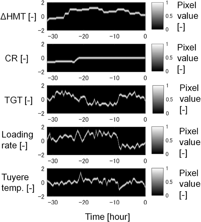
Input data used in 2D-CNN.

To predict the operators’ PCR control action, one of the three labels, i.e., increase PCR, decrease PCR, or hold PCR, was attached to each data. The label was determined by the sign of the PCR change within one hour.

Although operators manipulate PCR to maintain HMT near its target value, they do not always perform the correct actions. They sometimes perform incorrect control actions that increase the variation of HMT. If HMT is controlled by a CNN that imitates such operators’ wrong control actions, the HMT variance may become larger. Therefore, we overwrote the labels of wrong control actions with the label of holding PCR.

Figure 4 shows an example of the operators’ wrong control action, in which PCR was decreased at 0 h in spite of the decrease in the tuyere temperature during the past five hours. As a result, HMT decreased to more than 50°C below the target point. This large drop of HMT would have been mitigated if PCR had been increased at 0 h. Hence, the control action at 0 h is considered to be incorrect. Wrong control actions were defined as actions that resulted in ΔHMT lower than −10°C after a PCR decrease or ΔHMT higher than +10°C after a PCR increase, since it is likely the deviation of HMT would have been suppressed if PCR had been manipulated in the opposite direction to the actual operation. Considering the fact that the time constant of the step response of HMT to PCR is about 8 hours,³⁾ ΔHMT at 10 hours after the control action was used for the decision.

Fig. 4.

Example of wrong control action taken by operators. (Online version in color.)

2.3. Network Architecture of CNN

A CNN comprises three types of layers: a convolution layer, a pooling layer, and a fully connected layer. The convolution layer extracts the feature map from its input, and the fully connected layer outputs the weighted sum of the feature map downsized by the pooling layer. Figures 5(a) and 5(b) show the outline of the 2D-CNN and 1D-CNN, respectively. In this research, two types of input data were prepared as mentioned in Section 2.2, i.e., the 2D images of the trend of the input variables and the set of 1D vectors of the input variables. The former is fed to 2D-CNN while the latter is handled by 1D-CNN. In both CNNs, the final output is the probabilities of the three classes, i.e., increase PCR, decrease PCR, and hold PCR.

Fig. 5.

Outline of CNN structure. (a) 2D- CNN, (b) 1D-CNN. (Online version in color.)

2.3.1. 2D-CNN

In the convolution layer, the convolution operation is performed by a rectangular weight matrix (hereafter referred to as a filter), and a non-linear function is used for the activation. Let x be the input feature map of the convolution operation whose size is W×H×K and u be the output feature map of the convolution operation. The element u_ijm at position (i,j) in the m-th output feature map is calculated as follows.   

$$u_{ijm}={\sum }_{k=0}^{K-1}{\sum }_{p=0}^{F-1}{\sum }_{q=0}^{F-1}{A}_{pqkm}{x}_{Si+p,Sj+q,k}+b_m$$(2)

  

$$0\le i\le \frac{W-F}{S},0\le j\le \frac{H-F}{S}$$(3)

where p and q denote the indices of the horizontal and vertical positions of the filter. A_**km is the filter applied to the k-th input feature map used to generate the m-th output feature map, and its size is F×F. b_m is the bias of the m-th output feature map, and S is the stride of the convolution operation. The indices k and m are also referred to as channels.

In Eq. (2), the output feature map u is acquired by convolving the input feature map x with filters as shown in Fig. 5(a). To extract the local feature of the input feature map, the filter size F must be much smaller than W and H, i.e., the size of 2D images comprising the input feature map. The filter moves along the vertical axis and horizontal axis to generate the output feature map. The stride S has to be set smaller than F so that the convolution operation covers the whole area of the input feature map. After the convolution operation, the activation function f is applied.   

$$z_{ijm}=f\left(u_{ijm}\right)$$(4)

In this study, the ReLU function¹⁵⁾ was adopted as the activation function.

The pooling layer then performs down-sampling   

$$y_{ijm}=max\left(p,q\right)\in P_{ij}\mathrm{\hspace{0.17em} } z_{pqm},$$(5)

where P_ij is the neighborhood of the R×R square centered at position (i,j).

In this way, in the 2D-CNN, the input 2D images pass through several convolutional and pooling layers. The output feature maps are then weighted by the fully connected layers and the probabilities of the three classes, i.e., increase PCR, decrease PCR, and hold PCR, are calculated by a softmax function. Table 2 shows the network architecture of the 2D-CNN used in this work, where Conv, Pool, and Fc denote convolutional layer, pooling layer, and fully-connected layer, respectively. All the layers are connected in series.

Table 2. Network architecture of 2D-CNN.

Layer	Filter size	Stride	Output feature map size	Activation function	Number of parameters
Data			128×128×5
Conv1	3×3	1	126×126×4	ReLU	184
Pool1	2×2		63×63×4		0
Conv2	3×3	1	61×61×4	ReLU	148
Pool2	2×2		30×30×4		0
Conv3	2×2	1	29×29×4	ReLU	68
Pool3	2×2		14×14×4		0
Conv4	2×2	1	13×13×2	ReLU	34
Pool4	2×2		6×6×2		0
Fc1			1×6	ReLU	438
Fc2			1×3	softmax	21

This architecture of the 2D-CNN was determined to reduce the number of parameters for suppressing the over-fitting. As the number of parameters is increased, the parameters are adjusted to reproduce the sham correlation between the input variables and output variable in the training data caused by random noise. This over-fitting problem leads to the low prediction accuracy of other data such as validation data and test data. The over-fitting can be suppressed by reducing the number of parameters.

2.3.2. 1D-CNN

In the 1D-CNN, the input and output feature maps are 1D vectors as shown in Fig. 5(b). Convolving the input feature map x whose size is W×K with 1D filters derives the output feature map u. The convolution operation is performed only on the horizontal axis. The element u_im at position i in the m-th output feature map is calculated as follows.   

$$u_{im}={\sum }_{k=0}^{K-1}{\sum }_{p=0}^{F-1}{A}_{pkm}{x}_{Si+p,k}+b_m$$(6)

  

$$0\le i\le \frac{W-F}{S}$$(7)

where p is the index of the horizontal position of the filter. A_*km is the filter applied to the k-th input feature map to calculate the m-th output feature map, and its size is F×1. The 1D-CNN also comprises multiple convolutional layers and pooling layers, and the fully-connected layer is used to derive the probabilities of the three classes of PCR control actions. Table 3 shows the network architecture of the 1D-CNN employed in this study.

Table 3. Network architecture of 1D-CNN.

Layer	Filter size	Stride	Output feature map size	Activation function	Number of parameters
Data			64×5
Conv1	7×1	1	58×3	ReLU	129
Pool	2×1		29×3		0
Fc1			1×2	ReLU	176
Fc2			1×3	softmax	9

3. Validation of Operator Model with Actual Operation Data

We prepared 7200 points of pre-processed data for the 2D-CNN and 1D-CNN according to the procedure in Section 2.2. The five 2D images of the transition of the input variables shown in Fig. 3 were arranged in the channel direction and then input to the 2D-CNN, and the five 1D data vectors along the time axis were arranged in the channel direction and fed to the 1D-CNN. The first 5760 points were used for the training data, and the next 720 points were used to optimize the hyper-parameters of the CNNs, and the last 720 points were used as the test data to evaluate the prediction accuracies of the CNNs.

The stochastic gradient method was employed to optimize the parameters, i.e., the weights in the convolution layers and fully-connected layers. The cross-entropy error function was adopted for the loss function.   

$$E=-\frac{1}{N} {\sum }_{i=1}^N{\sum }_{c=1}^3{t}_{i,c}log{p}_{i,c}$$(8)

where N is the number of data points, and the suffix i represents the i-th data. t_i,c is the one hot label of class c, and p_i,c is the probability of class c derived from the CNNs, respectively.

Figures 6 and 7 show the validation results of the 2D-CNN and 1D-CNN, respectively. The red, green, and blue lines in the top row show the probabilities of increasing, decreasing, and holding PCR. The cross-entropy error E is shown in the top row. The red line in the bottom row shows the action score defined by   

$$S_a= p_1-p_2,$$(9)

where p₁ and p₂ are the probabilities of PCR increase and decrease by the CNN, respectively. In both the 2D-CNN and 1D-CNN, the action scores plotted by the red solid line and the actual control action marked by the blue circles in the bottom row showed similar trends.

Fig. 6.

Prediction result of 2D-CNN. (a) Probability of PCR action, (b) Comparison of actual PCR action and action score predicted by 2D-CNN. (Online version in color.)

Fig. 7.

Prediction result of 1D-CNN. (a) Probability of PCR action, (b) Comparison of actual PCR action and action score predicted by 1D-CNN. (Online version in color.)

The reason why the action score of the 2D-CNN changes slowly compared with the 1D-CNN is as follows. The network architecture of 2D-CNN comprises more convolution layers and pooling layers than 1D-CNN. It is because the architecture of 2D-CNN was determined to reduce the number of parameters for suppressing the over-fitting. Hence, the output of the 2D-CNN depends on the global features of the input images which do not change instantly.

In Figs. 6 and 7, the responses of the 2D-CNN and 1D-CNN are delayed when the actual operator control action was changed rapidly around day 8 and day 11. The reason for this delay in the CNN response compared to the operators’ control action is as follows. In addition to the input variables listed in Table 1, the operators also obtain information that is not recorded in the data, e.g., the color and particle size of the raw material, and they perform proactive control actions by using such information. For this reason, it is difficult to reproduce the operators’ control actions only by using the recorded data, and the response of the CNN can be slower than the actual action.

When the action score exceeded the upper threshold marked by the green dashed line in the bottom rows in Figs. 6 and 7, we decided the predicted control action was PCR increase. On the contrary, when the action score fell below the lower threshold, we judged the action was PCR decrease. The threshold was adjusted separately for the 2D-CNN and 1D-CNN so that the frequency of the predicted control actions, i.e., increase or decrease of PCR, agrees with the actual one. Tables 4 and 5 show the confusion matrices of the 2D-CNN and 1D-CNN, respectively. For example, the frequency of control action by 2D-CNN is 22.6%, i.e., the sum of 3.9%, 8.2%, 7.9%, and 2.6%, and that of the operators’ control action is 22.8%. Thus, the frequencies of the 2D-CNN and operator control actions are almost the same.

Table 4. Confusion matrix of 2D-CNN (N = 720).

Actual action by operators	Predicted action by CNN
	Increase	Hold	Decrease
Increase	3.9%	12.8%	0.0%
Hold	8.2%	61.1%	7.9%
Decrease	0.0%	3.5%	2.6%

Table 5. Confusion matrix of 1D-CNN (N = 720).

Actual action by operators	Predicted action by CNN
	Increase	Hold	Decrease
Increase	4.5%	7.5%	0.1%
Hold	7.9%	63.0%	6.5%
Decrease	0.0%	6.7%	3.9%

The accuracy of the operator model was 67.6% by 2D-CNN and 71.3% by 1D-CNN as shown in Tables 4 and 5. With both 2D-CNN and 1D-CNN, cases where the predicted control action was opposite to the actual action were limited to only 0.1%, showing the validity of the CNN-based approach. The 2D-CNN has a larger cross-entropy error than the 1D-CNN, and the 1D-CNN was superior to the 2D-CNN in terms of the percentage of correct actions. Therefore, the 1D-CNN was finally adopted in this study.

One of the reasons why the 1D-CNN showed better performance is that the number of parameters of the 2D-CNN is three times larger than that of the 1D-CNN, and as a result, over-fitting tends to occur in the 2D-CNN. Moreover, the 2D-CNN has multiple convolutional layers and pooling layers to minimize the influence of over-fitting, and this network architecture leads to a slow response to changes in the input variables. The accuracy of 2D-CNN could be improved by using more convolutional layers or adopting drop-out layers in future work. The accuracy may be further improved by incorporating the time-series characteristic of the input data by combining recurrent neural networks.¹⁶⁾

4. Evaluation of Operation Guidance System

The operator model was incorporated in the conventional operation guidance system²⁾ at an actual blast furnace. The conventional guidance system employs model predictive control (MPC) based on a transient model, and its control period is 30 minutes. The transient model considers the reaction and heat transfer phenomena in the furnace, and it is used to predict the future HMT assuming that the current operational conditions, e.g., coke ratio and blast temperature, are maintained in the future. MPC then outputs the appropriate control action to maintain HMT near the target value if the control deviation of HMT is predicted to be large.

One of the problems with the conventional MPC was that it sometimes provided incorrect control actions. Since the transient model in MPC only considers the influence of manipulated variables which can be manipulated by operators, it was difficult to output the appropriate control action when HMT deviated from the target value due to disturbances such as the changes in raw material characteristics. Therefore, we considered that the control accuracy of the guidance system could be improved by using the developed operator model which simulates the operators’ control actions.

We adopted the 1D-CNN model since it showed better prediction accuracy than the 2D-CNN. Table 6 shows the recommended control action, i.e., the final output of the guidance system, presented to the operators using the operator model and MPC. When the operator model or MPC indicates the control action of increasing or decreasing PCR, the guidance system adopts the control action as the recommended control action. If the MPC provides an output to increase the PCR and the operator model gives an output to decrease the PCR, the recommended control action is no PCR operation.

Table 6. Recommended control actions by operation guidance system.

Operator model	MPC using transient model
	Increase	Hold	Decrease
Increase	Increase	Increase	Hold
Hold	Increase	Hold	Decrease
Decrease	Hold	Decrease	Decrease

The operation guidance system using the operator model and MPC was evaluated in the actual operation. Figure 8(a) shows the control error of HMT for 12 days, and Fig. 8(b) compares the recommended control action with the operator model (red triangles) and the actual control actions by operators (blue circles). The operators mostly followed the guidance. Figure 8(c) shows the recommended control action by MPC alone. The MPC does not present any control actions around 5.3 day and 8.0 day as indicated by the green boxes. On the other hand, the recommended actions appear which are provided by the operator model in Fig. 8(b).

Fig. 8.

Evaluation of operation guidance system using operator model and transient model. (Online version in color.)

Figure 9 shows the trend of the input variables of the operator model and PCR at 5.1 day in Fig. 8. The origin of the horizontal axis is located at the moment when the recommended control action of decreasing PCR was presented. In the first row, the predicted HMT by the transient model is also shown by the green line. The transient model was not able to predict the rapid increase of HMT, and control action by MPC was holding PCR. In contrast, the operator model successfully presented the control action of PCR decrease. This control action seems to imitate the operators’ action in response to the increase of TGT and the tuyere temperature caused by the abnormal descent of materials.

Fig. 9.

Operational trend showing successful functioning of operator model when abnormal descent of materials occurred. (Online version in color.)

The blast furnace is filled with iron ore and coke, which normally descend smoothly through the furnace. However, the drag force of the ascending gas against the gravitational force of the material sometimes prevents a smooth descent. This phenomenon is called hanging. The transient model in MPC assumes the smooth descent of the solids in the furnace; it is difficult to predict the influence of hanging on changes in HMT. Therefore, the operator model is useful when the hanging occurs.

Figure 10 shows the operational trend at 8.5 day in Fig. 8. In this case, the type of iron ore was changed at -10 h. Since it is difficult for the transient model to consider the unmeasurable characteristics of iron ore such as the reducibility, the transient model was not able to predict the drop of actual HMT. However, the operator model properly directed the PCR increase, conceivably due to the decrease in the tuyere temperature during the previous eight hours.

Fig. 10.

Operational trend showing successful functioning of operator model when material characteristics changed. (Online version in color.)

The tuyere temperature tends to change ahead of HMT. It is because the tuyere temperature is influenced by the thermal status inside the furnace whereas HMT is measured outside the furnace. Interviews with operators indicate that they implement control actions to increase the PCR when the tuyere temperature drops. Therefore, the output of the operator model to increase the PCR in Fig. 10 can be attributed to the decrease in the tuyere temperature.

As demonstrated in these examples, the operator model can cope successfully with situations where the accuracy of the conventional guidance system deteriorates when the hanging of material occurs or the material characteristics change.

Figure 11 shows the effectiveness of the operator model based on an evaluation of HMT control errors 10 hours after the timing of guidance. The root mean square (RMS) of the control error was used to assess control performance. Figures 11(a) and 11(b) compare the HMT control error when the guidance was followed or not followed, respectively. The operators constantly monitor the guidance screen and perform control actions approximately every hour when the control action is necessary. Thus, we judged that the guidance was followed when the operators took control action within one hour after the recommended control action was presented. The RMS of the control error was smaller by 1.3°C when the guidance was followed. Figures 11(c) and 11(d) show the HMT control error when the guidance was followed or not followed, without using the operator model. The difference of the RMS of the control errors was only 0.1°C. The data period of Figs. 11(a) and 11(b) and that of Figs. 11(c) and 11(d) are the same. These results demonstrate that the operator model contributed to improving the control accuracy of HMT.

Fig. 11.

Comparison of HMT control accuracy when the guidance was followed or not followed (N=624). (Online version in color.)

5. Conclusion

In this study, an operator model that imitates the control actions of blast furnace operators was developed to improve the control accuracy of the hot metal temperature (HMT). Using time-series data of the operational trend as input, the operator model was created by a CNN to generate control actions that maintain a constant HMT. The predicted control actions matched the actual ones taken by operators in 71% of all cases. The operator model was then incorporated into the conventional operation guidance system, and it was evaluated in actual operation. As a result, the operation guidance system was able to present appropriate actions even in situations that were difficult to be addressed by the conventional operation guidance system, and the effect of reducing the variance of HMT was enhanced.

References

• 1)   M.  Naito,  K.  Takeda and  Y.  Matsui: ISIJ Int., 55 (2015), 7.
• 2)   Y.  Hashimoto,  Y.  Okamoto,  T.  Kaise,  Y.  Sawa and  M.  Kano: ISIJ Int., 59 (2019), 1573.
• 3)   Y.  Hashimoto,  Y.  Kitamura,  T.  Ohashi,  Y.  Sawa and  M.  Kano: Control Eng. Pract., 82 (2019), 130.
• 4)   V. R.  Radhakrishnan and  A. R.  Mohamed: J. Process Control, 10 (2000), 509.
• 5)   J.  Zeng,  C.  Gao and  H.  Su: Comput. Chem. Eng., 34 (2010), 1854.
• 6)   P.  Zhou,  D.  Guo,  H.  Wang and  T.  Chai: IEEE Trans. Neural Netw. Learn. Syst., 29 (2018), 4007.
• 7)   Y.  Hashimoto,  Y.  Sawa,  Y.  Kitamura,  T.  Nishino and  M.  Kano: ISIJ Int., 58 (2018), 2210.
• 8)   J.  de Castro,  A.  da Silva,  Y.  Sasaki and  J.  Yagi: ISIJ Int., 51 (2011), 748.
• 9)   H.  Saxén and  F.  Pettersson: ISIJ Int., 47 (2007), 1732.
• 10)   Z.  Ding,  J.  Zhang and  Y.  Liu: ISIJ Int., 57 (2017), 2022.
• 11)   A.  Díaz-Álvarez,  M.  Clavijo,  F.  Jiménez,  E.  Talavera and  F.  Serradilla: Transp. Res. Part F: Traffic Psychol. Behav., 56 (2018), 134.
• 12)   P.  Liu,  A.  Kurt and  Ü.  Özgüner: 17th Int. IEEE Conf. on Intelligent Transportation Systems (ITSC), IEEE, New York, (2014), 942.
• 13)   M.  Shimosaka,  K.  Nishi,  J.  Sato and  H.  Kataoka: 2015 IEEE Intelligent Vehicles Symp. (IV), IEEE, New York, (2015), 567.
• 14)   E.  Maggiori,  Y.  Tarabalka,  G.  Charpiat and  P.  Alliez: IEEE Trans. Geosci. Remote Sens., 55 (2017), 645.
• 15)   V.  Nair and  G. E.  Hinton: Proc. 27th Int. Conf. on Machine Learning, Omnipress, Wisconsin, (2010), 807.
• 16)   P.  Kittisupakorn,  P.  Thitiyasook,  M. A.  Hussain and  W.  Daosud: J. Process Control, 19 (2009), 579.