1. Introduction
To improve the performance of basic oxygen furnaces (BOFs), it is important to understand the complex dynamics in BOFs. In a BOF, supersonic gas jets of O2 are blown on a molten iron bath through a lance; consequently, impurities such as C, Si, Mn, and P are removed as CO–CO2 gas mixture and slag containing SiO2, MnO, and P2O5 through chemical reactions. The main role of BOFs is decarburization, which consumes approximately 100% of blown O2 in the main blowing stage, where the concentration of C in the bath is higher than approximately 0.3%.1) However, the details of the decarburization process are not well understood because of the complex interaction among many elementary processes, which involve the chemical reactions with the variable reaction rates coupled to the multiphase flow dynamics.
In order to understand the details of phenomena in BOFs, experiments have been conducted to observe and measure the inside of BOFs with a maximum temperature of over 2400 K2) and, more recently, simulations have been conducted using computational fluid dynamics (CFD). The main reaction sites for decarburization are typically presumed to comprise two zones, i.e., the impact zone, which is the surface of the cavity formed by the jet impinging on the molten iron bath, and the emulsion zone, where the droplets generated by the impinging jet, slag, and CO gas are mixed. For the emulsion zone, the mass percentage of metal droplets in the sampled emulsion has been experimentally investigated;3,4) however, the details are unclear owing to the complicated phenomena in the emulsion. For the impact zone, many studies have been conducted on the cavity formed by the jet. The relationship between the blowing conditions and the cavity shapes has been investigated by experiments with molten iron bath,5,6,7) cold models8,9,10,11,12) using water, glycerin, mercury, etc. and numerical simulations13,14,15,16) based on CFD. More recently, the cavity shape of a BOF was predicted by CFD, where the interaction among supersonic gas jets, molten iron, and slag was considered.17) However, the chemical reactions in the impact zone were not considered in the CFD models.
A reliable CFD model for the decarburization in the impact zone has not yet been established, although there are several related studies18,19,20) which consider decarburization with O2 (O2+2C=2CO) involving decarburization with CO2 (CO2+C=2CO) and post-combustion (CO+1/2O2=CO2), and studies21,22) which consider only decarburization with CO2. The chemical reaction models for the decarburization with O2 have not been sufficiently validated because the reaction rates of each of the three reactions, i.e., O2+2C=2CO, CO2+C=2CO, and CO+1/2O2=CO2, cannot be determined experimentally. For the decarburization with CO2, two CFD models (Cho et al.21) and Gao et al.22)) have been proposed so far, but neither of the two have considered both of the mass transfer in the gas-phase boundary layer and the interfacial chemical reaction rate, which would control the decarburization rate. Furthermore, their models were not validated under the high CO2 concentration condition, which is considered to be the case in actual BOFs from the model experiment with combustion in opposing flows of O2 and CO.23)
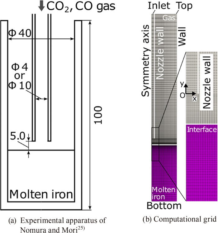
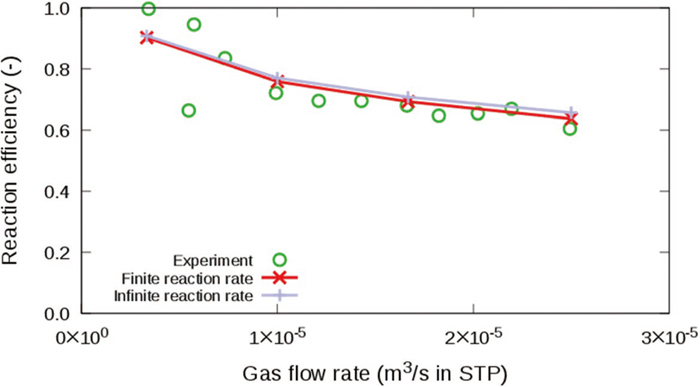
We herein propose a CFD solver, which fully couples governing continuum mechanics equations with a decarburization reaction model considering the mass transfer and the finite reaction rate on the gas-liquid interface, in order to elucidate the effects of each rate-limiting process. In this method, our pressure-based solver of mixed compressibility for two-phase flows24) was extended to treat reactive flows. The decarburization reaction model based on the model by Nomura and Mori25) was integrated into the CFD solver. The present method was validated by comparing the decarburization rates with those of Nomura and Mori’s element experiment.25)
2. Numerical Methods
2.1. Basic Equations
After adding mass conservation equations for chemical species to the governing equations of compressible/incompressible gas–liquid two-phase flows,24) we obtained the following equations:
• transport equation for the color function to track the gas-liquid interface:
|
D
α
l
Dt
=
α
l
α
g
ρ
g
D
ρ
g
Dt
+
α
g
ℛ
l,l-g
ρ
l
-
α
l
ℛ
g,l-g
ρ
g
| (1) |
• mass conservation equations for chemical species in gas and liquid phases:
|
∂
ρ
l
α
l
Y
l
X
∂t
+∇⋅(
ρ
l
α
l
Y
l
X
U
)
=-∇⋅
j
l
X
+
ℛ
l,l-g
X
| (2) |
|
∂
ρ
g
α
g
Y
g
X
∂t
+∇⋅(
ρ
g
α
g
Y
g
X
U
)
=-∇⋅
j
g
X
+
ℛ
g,l-g
X
| (3) |
• mass conservation equation:
|
∇⋅U=-
α
g
ρ
g
D
ρ
g
Dt
+
ℛ
l,l-g
ρ
l
+
ℛ
g,l-g
ρ
g
| (4) |
• momentum conservation equation:
|
∂ρU
∂t
+∇⋅(
ρUU
)
=-∇p-∇⋅τ+ρ∇G+
F
s
| (5) |
• energy conservation equation:
|
C
p
(
∂ρT
∂t
+∇⋅(
ρTU
)
)
=βT
Dp
Dt
-∇⋅q-τ:∇U+
Q
l-g
| (6) |
where
t (s) is the time,
α (–) the volume fraction of a phase (color function),
ρ (kg m
−3) the density,
Y (–) the mass fraction of the chemical species,
U (m s
−1) the velocity,
j (kg m
−2 s
−1) the diffusion flux of the chemical species,
ℛ
(kg m
−3 s
−1) the mass increase rate by the chemical reactions,
p (Pa) the pressure,
τ (Pa) the stress tensor,
G (m
2 s
−2) the gravitational potential,
Fs (N m
−3) the interfacial tension,
T (K) the temperature,
Cp (J kg
−1 K
−1) the specific heat at constant pressure,
β (K
−1) the coefficient of thermal expansion,
q (J m
−2s
−1) the heat flux,
Ql–g (J m
−3s
−1) the heat source by the decarburization reactions, and D/D
t the material derivative. Superscript X denotes the chemical species, whereas subscripts l, g, and l–g denote the liquid phase, gas phase, and interaction between the liquid and gas phases, respectively.
We assumed that the density of molten iron was constant, i.e., ρl,0=7000 kg m−3,26) and the density of gas was expressed by the equation of state for ideal gas. We used Fick’s, Newton’s, and Fourier’s laws in the conservation equations of mass of the chemical species, momentum, and energy as follows:
j
l
X
=-
ρ
l
α
l
D
l
∇
Y
l
X
,
j
g
X
=-
ρ
g
α
g
D
g
∇
Y
g
X
,
τ=-μ[
∇U+
(∇U)
T
-(∇⋅U)I/3
]
, and
q=-λ∇T
, respectively, where D (m2 s−1) is the diffusion coefficient, μ (Pa s) is the viscosity, λ (W m−1K−1) is the thermal conductivity. The phase-averaged material properties were calculated as φ=αlφl+αgφg, where φ denotes ρ, μ, λ, ρCp, or β. The diffusion coefficient of species X in molten iron was assumed to be constant, i.e.,
D
l
X
=Dl=7.0×10⁻⁹ m2 s−1.27) The diffusion coefficient in gas was calculated the Fuller–Schettler–Giddings correlation28) as the binary-diffusion coefficient of CO2–CO gas mixture. The viscosity of molten iron was assumed to be constant, i.e., μl=5×10⁻³ Pa s.15,29) The viscosity of gas was calculated from Sutherland’s law with coefficients obtained from the GRI-Mech 3.0 database.30) The thermal conductivity of molten iron was assumed to be constant, i.e., λl=40 W m−1 K−1.13,17,31) The thermal conductivity of the gas was calculated from the modified Eucken model.32) The specific heat at constant pressure of the molten iron was assumed to be constant, i.e., Cp,l=824 J kg−1 K−1.33) The specific heat at a constant pressure of the gas was calculated from the NASA polynomials.34) The interfacial force between the gas and the molten iron was calculated using the continuum surface force model35) with a constant coefficient of interfacial tension, i.e., σ=1.7 N m−1.36)
The mass increase rates
ℛ
l,l-g
X
and
ℛ
g,l-g
X
were calculated by a decarburization model described in Section 2.3.
2.2. Discretization and Solution Procedure
The basic equations listed in Section 2.1 were solved using a multistep solution procedure for pressure–velocity–density coupling, as in OpenFOAM.37) In the solution procedure, after solving the transport equation of the color function Eq. (1) by isoAdvector scheme,38) the intermediate densities ρ*, (ρl,0αl)*, and (ρgαg)* were calculated based on the mass conservation equations as follows:
|
ρ
*
=
ρ
n
-
Δt
V
∑
f
Φ
ρ,f
n
| (7) |
|
(
ρ
l,0
α
l
)
*
=
ρ
l,0
α
l
n
-
Δt
V
∑
f
Φ
ρ
l
,f
n
+
ℛ
l,l-g
n
| (8) |
|
(
ρ
g
α
g
)
*
=
ρ
g
n
α
g
n
-
Δt
V
∑
f
Φ
ρ
g
,f
n
+
ℛ
g,l-g
n
| (9) |
where the fluxes were calculated as
|
Φ
ρ,f
n
=
Φ
ρ
l
,f
n
+
Φ
ρ
g
,f
n
| (10) |
|
Φ
ρ
l
,f
n
=
ρ
l,0
Φ
α
l
,f
n
| (11) |
|
Φ
ρ
g
,f
n
=
ρ
g,f
n
(
Φ
f
n
-
Φ
α
l
,f
n
)
| (12) |
using
Φ
f
n
(m
3 s
−1) and,
Φ
α
l
,f
n
(m
3 s
−1), which are the entire and liquid volumetric flow rates at the cell face respectively. Subscript f denotes the cell face value, and Σ
f denotes the summation of the value over the cell faces. Using the intermediate densities, we obtained the mass fractions of chemical species
Y
l
X,n+1
and
Y
g
X,n+1
and the temperature
Tn+1 by solving the mass conservation equations for the chemical species and the energy conservation equation as follows:
|
(
ρ
l,0
α
l
)
*
Y
l
X,n+1
-
ρ
l,0
α
l
n
Y
l
X,n
Δt
+
1
V
∑
f
Y
l,f
X,n+1
Φ
ρ
l
,f
n
=∇⋅(
ρ
l
α
l
n+1
D
l
n+1
∇
Y
l
X,n+1
)
+
ℛ
l,l-g
X,n+1
| (13) |
|
(
ρ
g
α
g
)
*
Y
g
X,n+1
-
ρ
g
n
α
g
n
Y
g
X,n
Δt
+
1
V
∑
f
Y
g,f
X,n+1
Φ
ρ
g
,f
n
=∇⋅(
ρ
g
n
α
g
n+1
D
g
n+1
∇
Y
g
X,n+1
)
+
ℛ
g,l-g
X,n+1
| (14) |
|
C
p
(
ρ
*
T
n+1
-
ρ
n
T
n
Δt
+
1
V
∑
f
T
n+1
Φ
ρ,f
n
)
=
β
n+1
T
n+1
(
p
n
-
p
n-1
Δt
+
∑
f
p
f
n
Φ
f
n
-
p
n
∑
f
Φ
f
n
)
+∇⋅(
λ
eff
n+1
∇
T
n+1
)
+
Q
l–g
n+1
| (15) |
where the viscous dissipation term was neglected because we treat subsonic flows. After solving
Eqs. (13),
(14),
(15), the intermediate density
ρ
g
*
was calculated from the equation of state for ideal gas
ρ
g
*
=
p
n
/(
R
g
n+1
T
n+1
)
, where
Rg (J kg
−1 K
−1) is the gas constant of the mixture gas, and the pressure derivative of the density
ψ
g
(m
−2 s
2) was calculated as
ψ
g
n+1
=
(∂
ρ
g
/∂p)
n+1
=1/(
R
g
n+1
Tn+1), which were used to decouple the pressure, velocity, and density.
The coupled solution method of the pressure, velocity, and density is based on the fractional-step method. The momentum conservation equation was solved using a two-step time-advancement scheme as follows:
|
ρ
*
U
*
-
ρ
n
U
n
Δt
+
1
V
∑
f
U
f
n
Φ
ρ,f
n
-∇⋅[
μ
eff
n+1
(
∇
U
n
+
(
∇
U
n
)
T
-
2
3
I∇⋅
U
n
)
]=0
| (16) |
|
ρ
*
U
n+1
-
ρ
*
U
*
Δt
=
⟨
-∇
p
n+1
+
F
n+1
⟩
f→c
| (17) |
where the contribution of the surface tension and gravity
F is expressed as
|
F
n+1
=σ
κ
n+1
∇
α
n+1
+
ρ
*
∇G
| (18) |
In
Eq. (17), 〈〉
f→c represents an interpolation from the cell-face-centered point f to the cell-centered point c. The interpolation is expressed as
|
⟨ A ⟩
c
=
1
V
∑
f
(
S
f
⋅
A
f
)
(
x
f
-
x
c
)
| (19) |
where
A is an arbitrary vector,
Sf (m
2) the surface vector on the cell face, and
x (m) the position vector.
39) The mass conservation equation (
Eq. (4)) is discretized as follows:
|
1
V
∑
f
S
f
⋅
U
f
n+1
=-
α
g
n+1
ρ
g
*
D
ρ
g
n+1
Dt
+
ℛ
l,l-g
n+1
ρ
l,0
+
ℛ
g,l-g
n+1
ρ
g
*
| (20) |
Using
Eqs. (17) and
(20), the following pressure equation can be obtained:
|
1
V
∑
f
(
Δt
ρ
*
)
f
S
f
⋅∇
p
f
n+1
=
1
V
∑
f
S
f
⋅
U
f
*
+
1
V
∑
f
(
Δt
ρ
*
)
f
S
f
⋅
F
f
n+1
+
α
g
n+1
ρ
g
*
(
D
ρ
g
*
Dt
+
ψ
g
n+1
p
n+1
-
p
n
Δt
)
-
ℛ
l,l-g
n+1
ρ
l,0
-
ℛ
g,l-g
n+1
ρ
g
*
| (21) |
The material derivative term
D
ρ
g
*
/Dt
can be discretized as follows:
24)
|
D
ρ
g
*
Dt
=
ρ
g
*
-
ρ
g
n
Δt
+
1
V
∑
f
ρ
g,f
*
Φ
f
n
-
ρ
g
*
V
∑
f
Φ
f
n
| (22) |
The pressure
pn+1 was obtained by solving the pressure equation (
Eq. (21)). The velocity
Un+1 was obtained from
Eq. (17). The volumetric flow rate
Φ
f
n+1
=
U
f
n+1
·
Sf and density
ρ
g
n+1
were corrected as follows:
|
Φ
f
n+1
=
U
f
*
⋅
S
f
+
(
Δt
ρ
*
)
f
[
-
(
∇
p
n+1
)
f
+
F
f
n+1
]⋅
S
f
| (23) |
|
ρ
g
n+1
=
ρ
g
*
+
ψ
g
n+1
(
p
n+1
-
p
n
)
| (24) |
Subsequently, the density was updated to the following:
|
ρ
n+1
=
α
l
n+1
ρ
l,0
+
α
g
n+1
ρ
g
n+1
| (25) |
We developed a decarburization reaction model based on the model by Nomura and Mori,25) and integrated it into our CFD solver. The decarburization processes of molten iron by CO2 can be divided into two types of processes: chemical reactions at the gas–liquid interface and the mass transfer in the boundary layer. In the chemical processes, under the high concentration of C in molten iron, the rate-limiting reaction is assumed to be the direct reaction between CO2 and C at the gas–liquid interface described by:
|
CO
2
†
+
C
†
=2
CO
†
| (26) |
where superscript † indicates the chemical material at the interface. The dissolution reactions
CO
2
†
=C
†+2O
† and CO
†=C
†+O
† were excluded from the rate-limiting processes because the solubility of O in molten iron is low at high concentration of C. The reaction of
Eq. (26) may be divided into the elementary steps of dissociative adsorption of CO
2 and reaction between adsorbed O and C in the molten iron as follows.
where adsorbed O was expressed by O
*. Of two steps, the dissociative adsorption of CO
2 expressed by
Eq. (27) can be considered the rate-limiting step.
25,40) The reaction rate of the dissociative adsorption of CO
2,
Eq. (27), can be modeled
25,40) by:
|
r
CO
2
=s
p
¯
CO
2
,†
| (29) |
where
r
CO
2
(mol m
−2 s
−1) is the consumption rate of CO
2 per unit area,
p
¯
X
(atm) is the partial pressure of specie X in the standard atmosphere, and
s (mol m
−2 s
−1 atm
−1) is the forward reaction rate constant of
Eq. (27). The backward reaction rate was neglected because it is much smaller than the forward reaction rate at high concentration of C.
25) We used the reaction constant expressed by following equation.
40,41)
|
logs=3.007-1.049×
10
4
T
-1
| (30) |
The molar fluxes by mass transfer from the bulk to the gas–liquid interface, which move at the fluid velocity, N (mol m−2 s−1), are described as follows:
|
N
g→int
CO
2
=-
k
g
R
a
T
(
p
¯
CO
2
,†
-
p
¯
CO
2
)
+
p
¯
CO
2
,†
p
¯
†
(
N
g→int
CO
2
+
N
g→int
CO
)
| (31) |
|
N
g→int
CO
=-
k
g
R
a
T
(
p
¯
CO,†
-
p
¯
CO
)
+
p
¯
CO,†
p
¯
†
(
N
g→int
CO
2
+
N
g→int
CO
)
| (32) |
where the gas constant
Ra=8.20574×10
−5 m
3 atm K
−1 mol
−1,
k (m s
−1) is the mass transfer coefficient and
p
¯
†
=
∑
X
p
¯
X,†
is the pressure. The subscript of the molar flux,
g→int
, denote that the flux moves from the bulk of the gas to the interface. The bulk value
p
¯
X
was calculated as
p
¯
X
=
ρ
g
Y
g
X
(
R
a
/
M
g
X
)T
, where
M
g
X
is the molar mass. For the density
ρg, the mass fraction of chemical species
Y
g
X
, and the temperature
T, we used the value of the
nth step calculated by the CFD algorithm. The mass transfer coefficient
kg was calculated as
using the diffusion coefficient
Dg and distance
Δg which is one between the interface and the center of mass of the gas phase in the cell including the gas–liquid interface. Under the assumption that no accumulation of chemical species at the interface occurs, the consumption rate of CO
2 per unit area
r
CO
2
is equivalent to the flux in the bulk:
|
r
CO
2
=
N
g→int
CO
2
| (34) |
The following relations exist among the molar fluxes based on stoichiometric Eq. (26):
|
N
g→int
CO
=-2
N
g→int
CO
2
| (35) |
|
N
l→int
C
=
N
g→int
CO
2
| (36) |
The unknown variables
p
¯
CO
2
,†
,
p
¯
CO,†
were obtained by solving
Eqs. (31) and
(32) using
Eqs. (29),
(30), and
(33),
(34),
(35). We used the Levenberg–Marquardt method to solve the nonlinear simultaneous equations. In this way, the decarburization reaction model is integrated into the CFD solver and the decarburization rate can be calculated without using experimental results. It is in contrast to the analysis of decarburization by Nomura and Mori.
25) In their analysis, the mass transfer coefficient was estimated from the experimental decarburization rate using the empirical equation for the wall jet and the mass balances between the radial direction of the crucible and the direction normal to the interface.
The increase rates of the species by the chemical reactions in Eq. (26),
ℛ
, are expressed as follows:
|
ℛ
g,l-g
CO
2
=-
N
g→int
CO
2
M
g
CO
2
A
V
| (37) |
|
ℛ
g,l-g
CO
=-
N
g→int
CO
M
g
CO
A
V
| (38) |
|
ℛ
l,l-g
C
=-
N
l→int
C
M
l
C
A
V
| (39) |
where
V (m
3) is the volume of the cell,
A (m
2) is the interface area within the cell. The interface area was calculated using the interface reconstruction method from the color function based on the isoAdvector method.
38) The heat source of the chemical reaction in
Eq. (26),
Ql−g, is defined by
|
Q
l-g
=
ℛ
g,l-g
CO
2
M
g
CO
2
(
-Δ
H
2CO=
CO
2
+C
0
)
| (40) |
where the following enthalpy change
42) was used:
Δ
H
2CO=
CO
2
+C
0
= −144700.6 J mol
−1.
In addition to the reaction model described above, a reaction model which assumes infinite reaction rate for the dissociative adsorption of CO2 was used. In the model, we assumed that CO2 is completely consumed at the gas–liquid interface because of the infinite reaction rate. Therefore, substituting
p
¯
CO
2
,†
=0 and
p
¯
CO
2
=
ρ
g
RT
Y
g
CO
2
/
p
0
to Eq. (31), the molar flux of CO2 was calculated by:
|
N
g→int
CO
2
=
k
g
ρ
g
R
p
0
R
a
Y
g
CO
2
| (41) |
where
p0=101.325 kPa. The mass fraction
Y
g
CO
2
was implicitly treated as the value of the (
n+1)th step in solving the mass conservation equation for CO
2. The reaction model by Cho
et al.21) would give decarburization rates between that given by the models with finite and infinite reaction rates for the dissociative adsorption of CO
2 because it assumes thermodynamic equilibrium at the gas–liquid interface.
2.4. Algorithm Overview
The time-stepping procedure of the governing equations (Eqs. (1), (2), (3), (4), (5), (6)), including the calculation of the decarburization reaction rate, is summarized as follows:
1. The color function for the liquid phase
α
l
n+1
was obtained by solving Eq. (1) using the isoAdvector38) scheme. The color function for the gas phase was given by
α
g
n+1
=1−
α
l
n+1
.
2. The intermediate densities ρ*, (ρl,0αl)*, and (ρgαg)* were calculated using Eqs. (7), (8), (9).
3. The mass increase rates
ℛ
l,l-g
X,n+1
and
ℛ
g,l-g
X,n+1
and heat source
Q
l–g
n+1
associated with the decarburization reactions were calculated using the decarburization model, as in Eqs. (29)–(40).
4. The mass fractions of chemical species
Y
l
X,n+1
and
Y
g
X,n+1
were obtained by solving Eqs. (13) and (14) after updating the diffusion coefficient
D
g
n+1
.
5. The temperature Tn+1 was obtained by solving Eq. (15) after updating the specific heat at constant pressure
C
p
n+1
, the coefficients of thermal expansion βn+1, and thermal conductivity λn+1.
6. The density
ρ
g
*
and pressure derivative of the density
ψ
g
n+1
were updated using the equation of state for ideal gas.
7. The intermediate velocity U* was obtained from Eq. (16) after the viscosity was updated as μn+1.
8. The pressure pn+1 was obtained by solving Eq. (21).
9. The velocity Un+1, volumetric flow rate
Φ
f
n+1
, and densities
ρ
g
n+1
and ρn+1 were obtained using Eqs. (17) and (23), (24), (25).
10. The next time step was calculated based on steps 1 to 9 by updating the temporal index n with n+1.
The matrix solvers and spatial discretization schemes were selected considering the numerical stability and efficiency. The preconditioned conjugate gradient method was used for the pressure equation. Meanwhile, the preconditioned biconjugate gradient method was applied to solve the equations of energy and chemical species. The spatial derivatives for the diffusion terms were discretized using the second-order central-difference scheme. For the advection terms, the total variation diminishing scheme with the Sweby limiter43) was applied.