Visualising Martensite Phase Fraction in Bulk Ferrite Steel by Superimposed Bragg-edge Profile Analysis of Wavelength-resolved Neutron Transmission Imaging

Abstract

Bragg-edge neutron transmission imaging, a wavelength-resolved neutron imaging method, is a unique method for materials characterization. This method can quantitatively visualise various crystalline microstructural information in bulk material over several-centimetres with sub-millimetre spatial resolution. In various forms of crystalline information, the martensite phase fraction in ferritic steel is significant for the characterisation of, e.g., contact surface of an induction-hardened gear, dual phase (DP) steel used for automobiles, and the cutting edge of Japanese swords. However, the martensite phase fraction in a ferrite-martensite steel has not been measured using conventional Bragg-edge analysis methods because the entire neutron transmission spectral pattern of the α’-martensite phase corresponds to that of the α-ferrite phase. However, the Bragg-edge profile of the martensite phase is slightly broader than that of the ferrite phase. For these reasons, we developed a new method for measuring the ferrite/martensite phase fraction from the superimposed Bragg-edge (sBE) profile composed of both sharp α{110} Bragg-edge and broad asymmetric α’{110}-α’{101} Bragg-edge. As a result, two-dimensional imaging and computed tomography of the martensite phase fraction in ferrite-martensite steel were reasonably achieved. In addition, we observed the sBE analysis method to have numerous advantages such as reasonable accuracy (~5%), high precision and stability, and easy handling. Furthermore, we identified the suitability of an asymmetric crystal-lattice-plane-spacing distribution function for the determination of the α’{110}-α’{101} Bragg-edge profile, and found the blurred boundary by mixing unquenched and quenched regions in an induction-hardened steel rod.

1. Introduction

The martensite phase is the hardest microstructure in steel, owing to its fine microstructure and numerous defects.¹⁾ In several types of martensite crystal structures, the α’-martensite phase of the body centred tetragonal (BCT) crystal structure, which has a longer c-axis than the α-ferrite phase of the body centred cubic (BCC) crystal structure, is the most popular in industrial fields.²⁾ This martensite is present in various steels applied in fields ranging from industrial to cultural heritage applications, e.g., the contact surface of an induction-hardened gear,³⁾ dual phase (DP) and transformation-induced plasticity (TRIP) steels⁴⁾ used for automobiles, and the cutting edge of a Japanese sword.^5,6,7) For this reason, martensite has been frequently studied and characterised using electron microscopy,⁸⁾ X-ray diffraction⁹⁾ and neutron diffraction.¹⁰⁾ Particularly, with respect to the characterisation of a centimetre-sized material for actual use, neutron beam techniques bear the advantage of allowing for the investigation of the bulk-averaged information. This is attributed to the millimetre-centimetre gauge volume of neutron scattering owing to high penetration ability and centimetres beam size of a neutron beam. Bragg-edge neutron transmission imaging using a pulsed neutron source coupled with the time-of-flight (TOF) spectroscopy, which is one of the wavelength-resolved neutron imaging methods, is a new attractive method with neutrons.^11,12) This is because this method can quantitatively obtain bulk-averaged crystalline microstructural information for the neutron transmission path through a sample at each pixel position of a neutron TOF-imaging detector. In addition, this method exhibits certain advantages: sub-millimetre pixel size, and a visualisation area measuring approximately 100 mm × 100 mm, which is the detection area of neutron TOF-imaging detectors employing gas electron multiplier (GEM)¹³⁾ and micro pixel chamber (μPIC)¹⁴⁾ micropattern gas detectors used in our present study. This spatial imaging ability is an additional advantage for the actual use of engineering materials.

A lot of crystalline microstructural information can be evaluated using this method, e.g., crystalline phase fraction,^15,16,17,18) crystallographic texture,^11,19,20) crystallite size,¹¹⁾ macrostrain,^21,22,23,24) and microstrain/dislocation.²⁵⁾ The Bragg-edge wavelength broadening effect has frequently been used for the analysis and imaging of the martensite phase in ferrite-martensite steel.^{3,5,6,7,26,27,28,29)} The crystal structure of α’-martensite is close to that of α-ferrite, and the entire neutron transmission spectral patterns from these microstructures are almost the same.²⁶⁾ Therefore, a traditional crystalline phase fraction analysis method identifying the spectral patterns^15,16,17,18) cannot be applied to the ferrite-martensite phases. However, a single Bragg-edge profile caused by {110} and {101} diffractions of the α’-martensite phase is slightly broader than a single Bragg-edge profile caused by the {110} diffraction of the α-ferrite phase, which appears at the neutron wavelength of 0.405–0.415 nm.²⁶⁾ Therefore, previous Bragg-edge imaging studies have successfully conducted the visualisation of ferrite and martensite phases by profiling the small change of a single Bragg-edge wavelength broadening.^{3,5,6,7,26,27,28)} Furthermore, as a new approach, Su et al. quantitatively estimated the ferrite/martensite phase fraction, which was converted from the average value of crystal lattice plane spacing (d-spacing) distribution evaluated by the conventional single Bragg-edge profile analysis method.³⁾

However, the Bragg-edge imaging analysis of the ferrite/martensite phase fraction exhibits a technical limitation: when both the ferrite and martensite phases are present along the neutron transmission path, the neutron transmission spectrum at the wavelength ranging from approximately 0.405 to 0.415 nm has a superimposed Bragg-edge (sBE) profile owing to both {110} diffraction of the α-ferrite phase, and {110} and {101} diffractions of α’-martensite phase. In this case, the conventional single Bragg-edge profile analysis method²⁶⁾ cannot be applied because a sBE consists of three types of Bragg-edges/d-spacing distributions of α{110}, α’{110}, and α’{101}. For more accurate profiling, the contribution of these three components should be considered in the profile analysis. In addition, the conventional method evaluates only the full width at half maximum (FWHM) value of a single Gaussian d-spacing distribution, but not ferrite/martensite phase fraction. Furthermore, a d-spacing distribution composed of α’{110} and α’{101} should be represented by an asymmetric broad distribution but not a symmetric Gaussian distribution. After considering these effects, we propose a more optimised method for directly deriving the ferrite/martensite phase fraction from a sBE profile by analysing the ratio between an α{110} Bragg-edge profile and an α’{110}-α’{101} Bragg-edge profile with an improved profile function.

Therefore, in the present study, the sBE profile analysis method was established for the case where both ferrite phase and martensite phase were presenting along the neutron transmission path through a sample. In this method, the ferrite Bragg-edge and broadened martensite Bragg-edge were treated separately. As a result, this new approach could directly evaluate the ferrite/martensite phase fraction averaged over the neutron transmission path. The evaluations of this new approach were conducted using two types of samples: several types of steel plates with a thickness of 25 mm and comprising ferrite and martensite plates, and a cylinder with a diameter of 20 mm comprising ferrite at the centre and martensite on the exterior. Finally, we infer that the accuracy of ferrite/martensite phase fraction evaluated by this new method is sufficient for the tomography of ferrite/martensite phase fraction, that has not been deduced with respect to methods in previous studies. In addition, we report various new findings obtained through the development and the evaluation of the ferrite/martensite phase fraction imaging using the sBE analysis. For example, the Jorgensen-type asymmetric d-spacing distribution function is more suitable for profiling the Bragg-edge of the martensite phase of a SCM440 steel, and the boundary between the unquenched region and quenched region inside an induction hardened steel rod is unclear.

2. Experimental

The aim of the experiment is to indicate that quantitative estimation of ferrite/martensite phase fraction is feasible by using the sBE profile analysis. For this, accuracy, precision and imaging property of ferrite/martensite phase fraction measured by this new analysis method have to be evaluated by using samples with known quantities of ferrite and martensite phases. In this section, the prepared samples and the neutron TOF-imaging experiment methods are explained in detail.

2.1. Samples

We prepared SCM440 (Fe-1.04%Cr-0.62%Mn-0.41%C-0.17%Mo-0.17%Si) steels for ferrite, and quenched SCM440 steels for martensite. Figure 1 presents the schematic of samples composed of the ferrite and martensite phases. There are samples with two types of heat treatments. The first are the plate-type samples with a thickness of 25 mm, composed of five ferrite/martensite plates, as shown by Fig. 1(a). The dimensions of a single plate are 5 mm in thickness, and 50 mm × 50 mm in area. In this study, we assumed that a single quenched SCM440 plate had the martensite phase fraction of 100%. By combining five plates, we could prepare six types of martensite phase fractions for the neutron transmission path: 0%, 20%, 40%, 60%, 80% and 100%. In addition, for the plate-type samples, we prepared two types of martensite plates: a martensite plate receiving only quenching and with a Vickers hardness (HV) of 832, and a martensite plate receiving tempering after quenching and with a HV of 697. Using two types of martensite plates, we investigated the sBE analysis method for the different broadened Bragg-edge profiles. We studied the basic performance of the sBE analysis method using the plate-type samples. A neutron transmission spectrum was extracted from a 50 mm × 50 mm area because each quenched and tempered single plate had uniform spatial distributions of crystalline phase.

Fig. 1.

Schematic of samples composed of ferrite and martensite phases. (a) Examples of the plate-type samples. The ferrite and martensite plates of the 5 mm thickness were prepared and stacked to set various ferrite/martensite phase fractions for the neutron transmission path. (b) The rod-type sample, including ferrite and martensite phases, was prepared by induction hardening. The radius of the rod is 13 mm, and the radius of the ferrite region inside the rod is 8 mm because the martensite region exists to the width 5 mm from the outer surface. The rod-type sample was measured (b-1) along the axial direction for checking a cross-sectional distribution of ferrite/martensite phases, and (b-2) along the radial direction for evaluating the performance of the CT image reconstruction based on the sBE analysis method for the ferrite/martensite phase fraction. (Online version in color.)

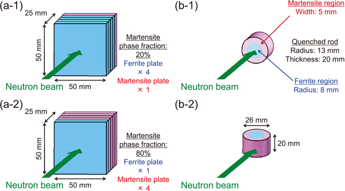
Figure 1(b) shows the second type of the sample, the rod-type sample, a simulating material of crankshaft in an automobile with a radius of 13 mm, and a thickness/height of 20 mm. The rod was subjected to induction hardening similar to our previous study.^26,27,28) As a result, the martensite phase of the HV of 629 was produced at the region up to a width of 5 mm from the outer surface of the rod. The ferrite region of the 8 mm radius remained at the rod centre. We measured the rod-type sample under two experimental setups: the direction of incident/transmitted neutron beams corresponding to that of the axial direction of the rod, and corresponding to that of the radial direction of the rod. This sample was measured for the evaluation of the performance of imaging and computed tomography (CT) of the ferrite/martensite phase fraction evaluated by the sBE analysis.

2.2. Pulsed Neutron Time-of-flight Imaging Instruments and Wavelength-resolved Neutron Transmission Imaging Experiments

The plate-type samples were measured using a pulsed neutron TOF-imaging method at the Hokkaido University Neutron Source (HUNS).^27,30) The electron linear accelerator for neutron production was operated under an electron energy of 33 MeV, electron pulse width of 4 μs, pulse repetition rate of 60 Hz, mean current of 60 μA and electron beam power of 2 kW. The neutron moderator was a decoupled/poisoned-type polyethylene moderator at ambient temperature.²⁷⁾ The 3.65Qc supermirror guide tube with a length of 3.8 m was installed in the neutron beamline.²⁷⁾ The neutron TOF-imaging detector was a GEM type detector¹³⁾ ‘THIN-GEM’ produced by Bee Beans Technologies Co., Ltd. in Japan. The pixel size was 0.8 mm, and the detection area was 100 mm × 100 mm. The TOF bin width was set to 5 μs. The samples were attached to the detector surface, and four samples were measured simultaneously owing to the large beam area size and the large detection area. The total neutron flight path length was 6.07 m, and the TOF/wavelength resolution at 0.4 nm was approximately 1% which was estimated through a {110} Bragg-edge profile evaluation of an α-Fe standard sample. The measurement time for neutrons transmitting the samples was 6 h, and the measurement time for neutrons without the samples was 6 h.

The rod-type sample was measured using a pulsed neutron TOF-imaging method at BL22 ‘RADEN’^31,32) at Materials and Life Science Experimental Facility (MLF) in Japan Proton Accelerator Research Complex (J-PARC). The beam power of the proton synchrotron during this experiment was 200 kW. RADEN was connected to a decoupled-type 20 K supercritical para-H₂ moderator. The B₄C ceramic collimator at 11.5 m from the neutron source was used to control both the neutron flux and neutron beam angular divergence. The open size of the collimator was 9 mm × 9 mm. The available neutron wavelength bandwidth was restricted from 0.1 nm to 0.5 nm by neutron choppers. The neutron TOF-imaging detector was a μPIC-based neutron imaging detector (μNID).¹⁴⁾ The pixel size was set to 0.8 mm, and the detection area was 100 mm × 100 mm. The TOF bin width was set to 10 μs. The sample was set on the CT stage at 200 mm from the detector. The total neutron flight path length was 23.86 m, and the TOF/wavelength resolution at 0.4 nm was approximately 0.2%. The collimator ratio, L/D, was 1373, and the umbra beam area size at the detector position was 89 mm × 89 mm. The rod-type sample was measured at rotating angles of 0°, 30°, 60°, 90°, 120°, and 150° in the CT (radial direction) experiment. The measurement time for neutrons transmitting the sample was 14 h for each projection, and 10 h for neutrons without the sample.

3. Superimposed Bragg-edge Profile Analysis Method

In this section, the sBE analysis method for the ferrite/martensite phase fraction analysis is explained. In addition, an improved d-spacing distribution function for more accurate Bragg-edge profiling for the martensite phase is discussed.

3.1. Basic Concepts of a Neutron Transmission Spectrum with a Bragg-edge Profile

Neutron transmission spectrum Tr(λ) measured at each detector pixel of a wavelength-resolved neutron imaging experiment is expressed as follows   

$$Tr\left(\lambda \right)=\mathrm{e}\mathrm{x}\mathrm{p}\left(-{\sum }_{P=1}^N\mathrm{\hspace{0.17em} }{\sigma }_P\left(\lambda \right)t_P\right)$$(1)

where λ is the neutron wavelength, P is the index of crystalline phase, N is the total number of crystalline phases, σ_P(λ) (cm²) is wavelength-dependent neutron total cross-section of crystalline phase P, and t_P (cm⁻²) is the areal density of the atomic number of the crystalline phase P. Traditionally, the crystalline phase fraction is evaluated using t_P^18,33) if there is a large difference in σ_P(λ)s. However, in the case of the combination of the BCC-structured ferrite phase and BCT-structured martensite phase, the difference in σ_P(λ)s between both phases is very small.²⁶⁾

Figure 2 shows a schematic of the d-spacing distribution of the α-ferrite phase, α’-martensite phase, and their superimposed distribution. The Bragg-edge of the ferrite phase at a neutron wavelength of 0.4 nm is caused by sharp symmetric distribution caused by {110} crystal lattice planes because the a-axis, b-axis, and c-axis in the crystal structure have the same parameters. Conversely, the Bragg-edge of the martensite phase at a neutron wavelength of 0.4 nm is caused by broad asymmetric distribution owing to the slightly small spacing’s {110} crystal lattice planes (a-axis and b-axis) and large spacing’s {101} crystal lattice planes (c-axis). The d-spacing distributions of the ferrite and martensite phases differ slightly. If both the ferrite and martensite phases exist along the neutron transmission path through a sample, a single but superimposed Bragg-edge is observed owing to a summation of d-spacing distributions as shown in Fig. 2. In such a situation, it is usually difficult to analyse the ferrite/martensite phase fraction using conventional methods. Therefore, in our present study, the difference between the wavelength broadening of the Bragg-edge of the ferrite and martensite phases is used to characterise each phase. When both the ferrite and martensite phases are present along the neutron transmission path, the superimposed data of sharp symmetric Bragg-edge spectrum and broad asymmetric Bragg-edge spectrum are measured. In the new data analysis method, the ferrite Bragg-edge and martensite Bragg-edge are separated from the superimposed Bragg-edge.

Fig. 2.

Schematic of d-spacing distribution of α-ferrite phase, α’-martensite phase and their superimposed distribution. Distribution of α-ferrite phase has sharp symmetric distribution due to {110} crystal lattice planes, and α’-martensite phase has broad asymmetric distribution due to {110} and {101} crystal lattice planes. (Online version in color.)

Here, the Bragg-edge profile Tr(λ) is expressed as follows.^15,34)   

$$Tr\left(\lambda \right)=\mathrm{e}\mathrm{x}\mathrm{p}\left(-\sigma \left(\lambda \right)\right)$$(2)

and   

$$\sigma \left(\lambda \right)={\sigma }_{\mathrm{b}\mathrm{a}\mathrm{s}\mathrm{e}}\left(\lambda \right)+{\sigma }_{hkl}\left(\lambda \right)\left[1-H\left(\lambda -2d\right)\right].$$(3)

Here, σ_base(λ) is the base total cross-section at a longer wavelength than a Bragg-edge of {hkl} diffraction, σ_hkl(λ) is the Bragg-edge cross-section at a shorter wavelength than the Bragg-edge of {hkl} diffraction, H(λ−2d) is the Heaviside step-function representing the Bragg “edge”, and d is crystal lattice plane spacing (d-spacing). The Bragg-edge is gradual: it exhibits wavelength broadening due to the instrumental resolution and the d-spacing distribution. Therefore, instead of 1−H(λ−2d), the Bragg-edge profile function B(λ−2d) is used.   

$$\sigma \left(\lambda \right)={\sigma }_{\mathrm{b}\mathrm{a}\mathrm{s}\mathrm{e}}\left(\lambda \right)+{\sigma }_{hkl}\left(\lambda \right)B\left(\lambda -2d\right).$$(4)

B(λ−2d) is a result of convolution between 1−H(λ−2d) and the broadening function D(λ−2d).¹⁵⁾   

$$B\left(\lambda -2d\right)=\left[1-H\left(\lambda -2d\right)\right]\otimes D\left(\lambda -2d\right).$$(5)

D(λ−2d) is equivalent to the profile function of a diffraction peak. Furthermore, B(λ−2d) or D(λ−2d) is separated to the instrumental broadening component, B₀(λ−2d) or D₀(λ−2d), and the sample (d-spacing distribution) broadening component, B₁(λ−2d) or D₁(λ−2d).²⁶⁾   

$$B\left(\lambda -2d\right)=B_0\left(\lambda -2d\right)\otimes B_1\left(\lambda -2d\right).$$(6)

  

$$D\left(\lambda -2d\right)=D_0\left(\lambda -2d\right)\otimes D_1\left(\lambda -2d\right).$$(7)

Although σ_base(λ) and σ_hkl(λ) of the martensite phase are usually equal to those of the ferrite phase, B₁(λ−2d) and D₁(λ−2d) of the martensite phase are broader than those of the ferrite phase.²⁶⁾ This difference is used to distinguish the martensite phase from the ferrite phase.

3.2. Improvement of a d-spacing Distribution Function for Single Bragg-edge Profile Fitting Analysis

In the present study and previous studies, the Jorgensen-type asymmetric function^15,35) has been used for instrumental resolution functions B₀(λ−2d) and D₀(λ−2d).^{3,5,6,7,12,25,26,27,36)}   

$$\begin{array}{l}{B}_0\left(\lambda -2d\right)=\\ {\displaystyle \frac{1}{2}}\text{erfc}\left(w_0\right)-{\displaystyle \frac{{\beta }_{0}exp\left(u_0\right)\text{erfc}\left(y_0\right)-{\alpha }_{0}exp\left(v_0\right)\text{erfc}\left(z_0\right)}{2\left({\alpha }_0+{\beta }_0\right)}}.\end{array}$$(8)

  

$$\begin{array}{l}{D}_0\left(\lambda -2d\right)=\\ {\displaystyle \frac{{\alpha }_0{\beta }_0}{2\left({\alpha }_0+{\beta }_0\right)}}\left[exp\left(u_0\right)\text{erfc}\left(y_0\right)+exp\left(v_0\right)\text{erfc}\left(z_0\right)\right].\end{array}$$(9)

Here,   

$$w_0=\frac{\lambda -2d}{\sqrt{2}{\sigma }_0},$$(10)

  

$$u_0=\frac{{\alpha }_0}{2}\left[{\alpha }_0{\sigma }_0^2+2\left(\lambda -2d\right)\right],$$(11)

  

$$v_0=\frac{{\beta }_0}{2}\left[{\beta }_0{\sigma }_0^2-2\left(\lambda -2d\right)\right],$$(12)

  

$$y_0=\frac{{\alpha }_0{\sigma }_0^2+\left(\lambda -2d\right)}{\sqrt{2}{\sigma }_0},$$(13)

and   

$$z_0=\frac{{\beta }_0{\sigma }_0^2-\left(\lambda -2d\right)}{\sqrt{2}{\sigma }_0}.$$(14)

In previous studies,^{3,5,6,7,12,25,26,27)} the Gaussian-type symmetric function with the standard deviation σ₁ has been used for d-spacing distribution functions B₁(λ−2d) and D₁(λ−2d).   

$$B_1\left(\lambda -2d\right)=\frac{1}{2}\text{erfc}\left(\frac{\lambda -2d}{\sqrt{2}{\sigma }_1}\right).$$(15)

  

$$D_1\left(\lambda -2d\right)=\frac{1}{\sqrt{2\pi }{\sigma }_1}\text{exp}\left(-\frac{{\left(\lambda -2d\right)}^2}{2{\sigma }_1^2}\right).$$(16)

However, as explained in the previous section and Fig. 2, a d-spacing distribution for a well-quenched martensite phase may become asymmetric because {101} crystal lattice plane spacing, which depends on the lattice parameter of c-axis in the crystal structure, can have a large d-value and a small frequency in d-spacing distribution as shown in Fig. 2. Therefore, the Jorgensen-type asymmetric function was used as d-spacing distribution functions B₁(λ−2d) and D₁(λ−2d) in the present study.   

$$\begin{array}{l}{B}_1\left(\lambda -2d\right)=\\ {\displaystyle \frac{1}{2}}\text{erfc}\left(w_1\right)-{\displaystyle \frac{{\beta }_{1}exp\left(u_1\right)\text{erfc}\left(y_1\right)-{\alpha }_{1}exp\left(v_1\right)\text{erfc}\left(z_1\right)}{2\left({\alpha }_1+{\beta }_1\right)}}.\end{array}$$(17)

  

$$\begin{array}{l}{D}_1\left(\lambda -2d\right)=\\ {\displaystyle \frac{{\alpha }_1{\beta }_1}{2\left({\alpha }_1+{\beta }_1\right)}}\left[exp\left(u_1\right)\text{erfc}\left(y_1\right)+exp\left(v_1\right)\text{erfc}\left(z_1\right)\right].\end{array}$$(18)

Here,   

$$w_1=\frac{\lambda -2d}{\sqrt{2}{\sigma }_1},$$(19)

  

$$u_1=\frac{{\alpha }_1}{2}\left[{\alpha }_1{\sigma }_1^2+2\left(\lambda -2d\right)\right],$$(20)

  

$$v_1=\frac{{\beta }_1}{2}\left[{\beta }_1{\sigma }_1^2-2\left(\lambda -2d\right)\right],$$(21)

  

$$y_1=\frac{{\alpha }_1{\sigma }_1^2+\left(\lambda -2d\right)}{\sqrt{2}{\sigma }_1},$$(22)

and   

$$z_1=\frac{{\beta }_1{\sigma }_1^2-\left(\lambda -2d\right)}{\sqrt{2}{\sigma }_1}.$$(23)

σ, α, and β in the Jorgensen-type entire Bragg-edge profile function B(λ−2d) have the following relationship for parameters in B₀(λ−2d) and B₁(λ−2d):   

$${\sigma }^2={\sigma }_0^2+{\sigma }_1^2,$$(24)

  

$$\frac{1}{\alpha }=\frac{1}{{\alpha }_0}+\frac{1}{{\alpha }_1},$$(25)

and   

$$\frac{1}{\beta }=\frac{1}{{\beta }_0}+\frac{1}{{\beta }_1}.$$(26)

Therefore, the Jorgensen-type function was used for both B₀(λ−2d_hkl) and B₁(λ−2d_hkl) in the present study. This is effective for the flexible description of various d-spacing distributions. As a result, more accurate fitting is expected for a complicated Bragg-edge profile with asymmetric Bragg-edge wavelength broadening owing to {110} and {101} diffractions of the martensite phase of SCM440.

3.3. Superimposed Bragg-edge Profile Fitting Analysis and its Limitation with Required Assumption

For the samples measured in this study, both the ferrite and martensite phases existed along a neutron transmission path. For more accurate profile fitting toward sBE owing to both the sharp symmetric Bragg-edge of ferrite and broad asymmetric Bragg-edge of martensite, and the direct derivation of the ferrite/martensite phase fraction, we developed and applied the sBE profile fitting analysis method. The superimposed Bragg-edge profile function B(λ−2d) for Eq. (4) can be expressed as follows.   

$$B\left(\lambda -2d\right)=\left(1-R\right)B_{\mathrm{f}\mathrm{e}\mathrm{r}}\left(\lambda -2d\right)+R\mathrm{\hspace{0.17em} }{B}_{\mathrm{m}\mathrm{a}\mathrm{r}}\left(\lambda -2d\right),$$(27)

where   

$$B_{\mathrm{f}\mathrm{e}\mathrm{r}}\left(\lambda -2d\right)=B_0\left(\lambda -2d\right)\otimes B_{1,\mathrm{f}\mathrm{e}\mathrm{r}}\left(\lambda -2d_{\mathrm{f}\mathrm{e}\mathrm{r}}\right),$$(28)

and   

$$B_{\mathrm{m}\mathrm{a}\mathrm{r}}\left(\lambda -2d\right)=B_0\left(\lambda -2d\right)\otimes B_{1,\mathrm{m}\mathrm{a}\mathrm{r}}\left(\lambda -2d_{\mathrm{m}\mathrm{a}\mathrm{r}}\right).$$(29)

B_fer(λ−2d) is the Bragg-edge profile comprising instrumental resolution component B₀(λ−2d) and d-spacing distribution component owing to the ferrite phase B_1,fer(λ−2d_fer). B_mar(λ−2d) is the Bragg-edge profile comprising instrumental resolution component B₀(λ−2d) and d-spacing distribution component owing to the martensite phase B_1,mar(λ−2d_mar). R is the fraction of the martensite phase (0–1).

The procedure of an actual data analysis is as follows.

• σ₀, α₀, β₀ and d (=d_fer) in B₀(λ−2d) are determined using the standard Bragg-edge data of the ferrite phase B_fer(λ−2d). We assume that the experimentally observed Bragg-edge profile of the ferrite phase B_fer(λ−2d) is equal to the Bragg-edge profile owing to the instrumental resolution B₀(λ−2d). This assumption has been used as in previous studies.^{3,5,6,7,26,27,28)}

• σ_1,mar, α_1,mar, β_1,mar, and d_mar - parameters in B_1,mar(λ−2d_mar) - are determined using the standard Bragg-edge data of the martensite phase B_mar(λ−2d). We assume that instrumental resolution component B₀(λ−2d) between the ferrite and martensite phases remains unchanged.

• The sBE data is analysed by profile fitting using Eqs. (2), (4), and (27) with the known information B_fer(λ−2d) = B₀(λ−2d) and B_mar(λ−2d). B_fer(λ−2d) and B_mar(λ−2d) are fixed during data analysis. The martensite phase fraction R can be finally determined through analysis.

The need to measure the standard Bragg-edge data of both phases of ferrite and martensite before the sBE analysis limits this method. Here, we guess that the sBE analysis is robust for strain/stress effect. This is because the magnitude of Bragg-edge broadening due to martensite phase²⁶⁾ is 10 times larger than that due to plastic deformation.³⁷⁾ Thus, the evaluation of ferrite/martensite phase fraction using the Bragg-edge imaging method is feasible owing to the sBE analysis.

4. Results and Discussion

4.1. Measured Neutron Transmission Spectra

Figure 3 shows the experimental results of the Bragg-edge spectra of the plate-type samples composed of ferrite, quenched martensite, and quenched-tempered martensite. These data were obtained from five plates. Figure 3(a) shows the entire pattern of the neutron transmission spectra of ferrite, tempered martensite, and quenched martensite. The shapes of the neutron transmission spectra from 0.3 nm to 0.4 nm for ferrite and two types of martensite steels differ. This change is caused by differences in crystal orientation distribution, that is, crystallographic texture.^11,19) Conventionally, it is important for crystalline phase fraction analysis that the Bragg-edge height and wavelength patterns of analysed crystalline phases such as ferrite (or martensite) and austenite differ, because the pattern decomposition is necessary for the quantification of each crystalline phase.^15,16,17,18) However, the pattern decomposition is not usable in the ferrite-martensite case because the spectral pattern between ferrite and martensite is almost the same. Therefore, in our present study, it is utilized that the Bragg-edge profile of martensite is broader than that of ferrite. Figure 3(b) shows the α{110} Bragg-edge profile of the ferrite phase, and α’{110}-α’{101} Bragg-edge profiles of the tempered and quenched martensite phases. The Bragg-edge wavelength broadening of martensite steels exceeds that of ferrite steel. In addition, the Bragg-edge wavelength broadening of quenched martensite (HV 832) exceeds that of tempered martensite (HV 697). Similar Vickers hardness dependence of Bragg-edge wavelength broadening was also observed in a previous study.²⁶⁾ Figures 3(c) and 3(d) show the profile changes in α{110} and α’{110}-α’{101} sBE of various α/α’phase fractions. The sBE profile broadens depending on the martensite phase fraction. This profile change is analysed using Eqs. (2), (4), and (27), and the martensite phase fraction is derived.

Fig. 3.

Bragg-edge neutron transmission spectra of the plate-type samples composed of ferrite, quenched/tempered martensite, and quenched martensite, measured at HUNS. These data were obtained from five plates. (a) Bragg-edge neutron transmission spectra of ferrite, tempered martensite, and quenched martensite. (b) α{110} Bragg-edge of ferrite, and α’{110}-α’{101} Bragg-edges of tempered martensite and quenched martensite. (c) α{110} and α’{110}-α’{101} sBE of various phase fractions of ferrite and tempered martensite. (d) α{110} and α’{110}-α’{101} sBE of various phase fractions of ferrite and quenched martensite. (Online version in color.)

Figure 4 shows the Bragg-edge profiles of ferrite, ferrite-martensite, and martensite phases of the rod-type sample. The standard Bragg-edge data of the ferrite phase was obtained from the axial direction measurement shown by Fig. 1(b-1). The sBE data of the ferrite and martensite phases were obtained from the rod centre position of the radial direction measurement shown by Fig. 1(b-2). The martensite phase fraction at the rod centre in the radial direction experiment is approximately 38% because the total thickness along the neutron transmission path of ferrite is 16 mm, and the total thickness along the neutron transmission path of martensite is 10 mm. Finally, the standard Bragg-edge data of the martensite phase was obtained from the radial direction measurement shown by Fig. 1(b-2). The sample thickness for the neutron transmission path between these data is different because it depends on both the sample direction and pixel position. Therefore, the vertical axis of Fig. 4 is normalised by multiplying the measured neutron transmission value by an exponential function with the exponent chosen to adjust the difference in sample thickness. Here, we selected the data of the 26 mm thickness as the standard data. The Bragg-edge profile becomes broader depending on the martensite phase fraction as well as the plate-type samples. In addition, after checking the data, we confirmed that the shapes of the entire neutron transmission spectra of the martensite phase, which can be changed by crystallographic texture, were not changed by the sample directions (axial or radial) and rotation angles in the radial direction experiments. This result is consistent with results in previous reports.^28,38) Therefore, we conducted the CT image reconstruction of martensite phase fraction.

Fig. 4.

Bragg-edge neutron transmission spectra of the rod-type sample, measured at RADEN. Three types of data are shown; standard α{110} Bragg-edge of the ferrite phase obtained by the axial direction measurement, α{110} and α’{110}-α’{101} sBE composed of ferrite phase (16 mm thickness) and martensite phase (10 mm thickness) obtained by the radial direction measurement, and standard α’{110}-α’{101} Bragg-edge of the martensite phase obtained by the radial direction measurement. The vertical axis is normalised by multiplying the measured neutron transmission value by an exponential function with the exponent chosen to adjust the difference in sample thickness. (Online version in color.)

4.2. Improvement of the Single Bragg-edge Profile Fitting Using the Jorgensen-type Asymmetric d-spacing Distribution Function

Our previous study measuring S45C, which has lower Vickers hardness and sharper Bragg-edge than SCM440, used the Gaussian-type symmetric d-spacing distribution function. Before the sBE analysis, we investigated the effect of the Jorgensen-type asymmetric d-spacing distribution function, Eqs. (17), (18), (19), (20), (21), (22), (23). Figure 5 shows the results of profile fitting toward a standard Bragg-edge data of martensite phase of the rod-type sample measured along the radial direction, using the Gaussian-type function and the Jorgensen-type function. Although fitting using the Gaussian-type d-spacing distribution was sufficient for the Bragg-edge wavelength broadening of martensite phase of S45C,²⁶⁾ Fig. 5(a) shows that the Gaussian-type symmetric d-spacing distribution is not sufficient for the asymmetric Bragg-edge wavelength broadening owing to α’{101} diffraction of martensite phase of SCM440. Conversely, Fig. 5(b) shows that the Jorgensen-type asymmetric d-spacing distribution can be further fitted for the asymmetric Bragg-edge wavelength broadening owing to α’{101} diffraction of martensite phase of SCM440. Therefore, we found more accurate Bragg-edge profile fitting function using the Jorgensen-type asymmetric d-spacing distribution, Eqs. (17), (18), (19), (20), (21), (22), (23). Hereafter, the sBE analysis method adopts this type of single Bragg-edge profile fitting function.

Fig. 5.

Improvement of the single Bragg-edge profile fitting using the Jorgensen-type instrumental resolution function and the Jorgensen-type d-spacing distribution function. The experimental data is a standard Bragg-edge obtained from martensite phase measured along the radial direction of the rod-type sample of SCM440, measured at RADEN. (a) The d-spacing distribution function is the symmetric Gaussian type. (b) The d-spacing distribution function is an asymmetric Jorgensen type. (Online version in color.)

4.3. Ferrite/martensite Phase Fraction Derived by the Superimposed Bragg-edge Profile Analysis Using Standard Bragg-edge Profiles

We discuss the accuracy and precision of the analysis results of the ferrite/martensite phase fraction derived by the sBE analysis. The data shown in Figs. 3(c) and 3(d) were used. Before the sBE analysis, the determination of the standard Bragg-edge profiles of both the ferrite and martensite phases is necessary. Figure 6(a) shows the standard Bragg-edge profile determination for the ferrite phase, the tempered martensite phase, and the quenched martensite phase. The fitting curves are well fitted to the experimental data shown by Fig. 3(b). Next, the sBE profiles obtained from the plate-type samples composed of both ferrite and martensite phases shown by Figs. 1(a-1) and 1(a-2) were analysed based on the ferrite and martensite standard Bragg-edge profiles presented by Eq. (27). Figure 6(b) shows examples of the sBE fitting toward the data of martensite phase fraction of 40%. Figure 6(b) shows two types of data: tempered martensite and quenched martensite data. The sBE fittings were well conducted; we derived the martensite phase fraction, R, through the sBE fitting presented by Eq. (27).

Fig. 6.

(a) Determination of the standard Bragg-edge profiles of ferrite phase, tempered martensite phase, and quenched martensite phase, which data are shown by Fig. 3(b) measured at HUNS. These profiles are used for the sBE fitting analysis of the ferrite/martensite phase fraction. (b) sBE analyses for tempered martensite phase fraction of 40%, and quenched martensite phase fraction of 40%. (c) Summary of analysis results of martensite phase fraction evaluated from the Figs. 3(c) and 3(d) data. (Online version in color.)

Figure 6(c) shows the results of derived martensite phase fraction, R, for twelve sets of data of sBE obtained from ferrite-martensite combination plate samples measured at HUNS. The horizontal axis represents the actual martensite phase fraction along the neutron transmission path. These values are immediately calculated from the number of ferrite plates and martensite plates. The vertical axis refers to the martensite phase fraction, R, derived from the sBE analysis. If the derived values exist on the black solid line in the figure, the actual martensite phase fractions are derived using our proposed method.

• Evaluation of accuracy: The derived values of both the tempered martensite samples and the quenched martensite samples are distributed around the actual values. Here, we evaluate the uncertainty of the derived martensite phase fraction, U, using the following equation.   

$$U=\frac{1}{M}{\sum }_{i=1}^M\left|R_i-R_i^{\text{actual}}\right|,$$(30)

where, M is the total number of the derived martensite phase fraction (M = 12), R_i is the experimentally derived martensite phase fraction of i-th data, and $R_i^{\text{actual}}$ is the actual martensite phase fraction of the i-th data. In the present study, U was 0.048 (4.8%). This value is comparable to the value of a ferrite/austenite phase fraction analysis using RITS,¹⁸⁾ although the sBE analysis method is easier in terms of data analysis handling, compared with RITS, which addresses a lot of microstructural parameters. Here, we discuss an estimated reason for the value of U. The trend of Fig. 6(c) was unchanged when three ferrite plates and three martensite plates were selected and used to determine the standard Bragg-edge profiles of both the ferrite and martensite phases; five ferrite plates and five martensite plates were used for Fig. 6. Therefore, the uncertainty, U, might be caused by the analysed data with systematic errors due to a limited instrumental resolution of the HUNS beamline. This analysis method is applied to a wavelength range that is significantly narrower than that of RITS, and has to detect significantly small changes in Bragg-edge wavelength broadening, as shown by Figs. 3(c) and 3(d). It is difficulty for this method from a viewpoint of accuracy. Incidentally, in our other experimental studies, the accuracy in experiments with a neutron grid collimator¹⁸⁾ suppressing background neutrons scattered from a sample did not change. We therefore consider the Bragg-edge profile regarding the wavelength direction (wavelength resolution) to be more important for crystalline phase quantification in this method than the entire neutron transmission intensities corrected by a neutron grid collimator.

• Evaluation of precision: The sBE analysis method provides a small analysis error. We do not show the error bar in Fig. 6(c) because the martensite phase fractions were stably derived with high precision. In other words, the same value of martensite phase fraction was always derived using any initial parameters in profile fitting procedure. As a result, lengths of error bars are smaller than the size of plots in Fig. 6(c). This stability with high precision is advantageous, compared with ferrite/austenite phase fraction analysis using RITS with low precision/low analysis stability but high accuracy/correct value derivation.¹⁸⁾

Therefore, the sBE analysis method could provide the ferrite/martensite phase fraction directly from a Bragg-edge spectrum. In addition, data analysis results showed that this method had numerous advantages such as reasonable accuracy, high precision, easy handling, and high stability.

4.4. Computed Tomography Image Reconstruction of Ferrite/martensite Phase Fraction

For the analysis and imaging of martensite phase fraction of the rod-type sample by the sBE analysis, we first determined the standard Bragg-edge profile of the ferrite and martensite phases. Figure 7(a) shows the single Bragg-edge profile fitting toward a Bragg-edge of ferrite phase measured at the central region in the axial direction experiment of the rod-type sample. The determination of the standard Bragg-edge profile of the martensite phase was performed as shown in Fig. 5(b). Using two standard Bragg-edge profiles of the ferrite and martensite phases, the sBE analyses were conducted as shown in Fig. 7(b). Each fitting was reasonably performed; therefore, the martensite phase fraction can be derived through the sBE analysis.

Fig. 7.

(a) Determination of the standard Bragg-edge profile of the ferrite phase of the rod-type sample. The Bragg-edge spectrum was obtained from the axial direction experiment. (b) sBE analysis toward the data of martensite phase fraction of 38%, obtained at the rod centre of the radial direction experiment. (Online version in color.)

Next, the martensite phase fractions at each pixel position in the rod-type sample were visualised using pixel-by-pixel sBE analyses. The computation time per pixel was less than 2 seconds when a common desktop computer (12-core 3.46 GHz CPU, 24 GB RAM) was used. This is because the sBE analysis is applied to a quite narrow wavelength range. It is advantage of the sBE analysis that a special computing system such as supercomputer is not necessary. Figure 8 shows the imaging result of the martensite phase fraction of the rod-type sample in (a) the axial direction setup and (b) the radial direction setup. The pixel size is 0.8 mm × 0.8 mm. Figure 8(c) shows the position dependence of the martensite phase fraction from the centre of the rod to its exterior surface, in the radial direction experiments. The plot data were averaged over the vertical direction from y = − 6.4 mm to y = + 6.4 mm and the rotation angles, 0°, 30°, 60°, 90°, 120°, and 150°, and also averaged axial-symmetrically, for Fig. 8(b). The black solid line represents the estimated values of the martensite phase fraction averaged over the neutron transmission path, calculated from the geometry condition that the martensite phase exists at the outer surface in the region of the 5 mm width and the ferrite phase exists at the centre in the region of the 8 mm radius. As a result, in both the axial direction experiment and the radial direction experiment, the 100% martensite phase region was observed at the 5 mm width from the outer surface of the rod-type sample. The region composed of the 100% ferrite phase was observed at the 8 mm radius at the centre region of the rod-type sample. Conversely, according to Figs. 8(a) and 8(c), the spatial boundary between the ferrite and martensite phases appears to be unclear.

Fig. 8.

Two-dimensional imaging of martensite phase fraction obtained by the sBE analysis of the rod-type sample measured at RADEN. (a) Axial direction. (b) Radial direction. (c) Martensite phase fractions derived at each position of the rod-type sample measured along the radial direction, compared with the values estimated from the geometry. The geometry is assumed to be the radius of the ferrite region (8 mm), and the martensite width from the outer surface (5 mm). (Online version in color.)

Finally, we conducted the CT image reconstruction from the position-dependent martensite phase fraction data of the radial direction experiments with the rotation angles 0°, 30°, 60°, 90°, 120°, and 150°. The used CT image reconstruction algorithm is ML-EM (maximum likelihood-expectation maximisation).³⁹⁾ The number of projection data in a certain rotation angle is 33. The number of rotations is 12, which corresponds to every 30°. The reconstructed CT image is visualised in 51 × 51 pixels. The data in Fig. 8(c) were used as the projection data. Figure 9(a) shows the result of the CT image reconstruction of the martensite phase fraction in the rod-type sample. Figure 9(b) shows the radial dependence of the martensite phase fraction of the CT image shown in Fig. 9(a), and the two-dimensional image obtained from the axial direction experiment shown in Fig. 8(a). Figure 9(b) is the plot data after the circular averaging. Based on Fig. 9, we identified certain important evaluation points for Figs. 8(a) and 9(a) as follows.

Fig. 9.

(a) CT image of the martensite phase fraction in the rod-type sample, reconstructed from the data between y = − 6.4 mm and y = + 6.4 mm of Fig. 8(b). (b) Comparison between the martensite phase fractions of the CT image (Fig. 9(a)), and the axial direction image (Fig. 8(a)). (Online version in color.)

• Figure 9(a) is consistent with Fig. 8(a).

• The martensite phase is 100% on the outer region, and 0% at the central region.

• At 8 mm from the rod centre, which is an estimated boundary between the ferrite and martensite regions, the martensite phase fraction corresponds to 50%. It is shown by an arrow in Fig. 9(b). Therefore, the 8 mm position corresponded to the boundary between the ferrite and martensite regions.

• The boundary between the ferrite and martensite regions is unclear, as discussed in the previous paragraph. This gradual boundary distribution has also been observed in a previous study²⁸⁾ which applies the same rod sample and visualises the FWHM of d-spacing distribution using the microchannel plate (MCP) type neutron TOF-imaging detector with ultrafine pixels of 55 μm.⁴⁰⁾ This gradual boundary may result from the spatial blurring of induction hardening/quenching because such a gradual boundary is not observed in a steel rod with a clear boundary between crystalline phases.¹⁸⁾

• The martensite phase fractions from 0 mm to 8 mm in the radius of the CT image are lower than those of the axial direction image. This is because the CT image was reconstructed from the data of Fig. 8(c), which were averaged from y = − 6.4 mm to y = + 6.4 mm of Fig. 8(b). Although the martensite phase exists near the rod centre region at y = − 10 mm and y = + 10 mm in Fig. 8(b), the data of these vertical outer regions were not included in the CT image reconstruction. However, such data were included in the axial direction experiment, Fig. 8(a). Therefore, the martensite phase fractions of the axial direction image from 0 mm to 8 mm in radius are higher than those of the CT image. To check these estimations, we conducted CT image reconstruction using the full vertical data from y = − 10 mm to y = + 10 mm of Fig. 8(b). Figure 10 shows the tomographic reconstruction result. The martensite phase fractions from 0 mm to 8 mm in the radius of the CT image are close to those of the axial direction image. In other words, Fig. 9 shows that a cross-sectional distribution of the martensite phase fraction at a certain layer can be non-destructively visualised via tomography. Conversely, the reason underlying the presence of the martensite phase near the rod centre region at y = − 10 mm and y = + 10 mm in Fig. 8(b) was not identified, despite the cutting of the rod sample after quenching.

Fig. 10.

(a) CT image of the martensite phase fraction in the rod-type sample, reconstructed from the full vertical data between y = − 10 mm and y = + 10 mm of Fig. 8(b). (b) Comparison between the martensite phase fractions of the CT image (Fig. 10(a)), and the axial direction image (Fig. 8(a)). (Online version in color.)

Therefore, we concluded that the two-dimensional imaging and CT image reconstruction of the martensite phase fractions in the bulk ferrite steel can be performed using wavelength-resolved neutron imaging and sBE analysis.

5. Conclusions

The Bragg-edge neutron transmission imaging can quantitatively visualise various crystalline microstructural information over several-centimetres with sub-millimetre spatial resolution in bulk material non-destructively. In the present study, the sBE analysis method was developed for the ferrite/martensite phase fraction imaging, which could not be achieved by conventional Bragg-edge analysis methods. We focus on the small profile change of α{110}-α’{110}-α’{101} Bragg-edges between the α-ferrite phase and α’-martensite phase. As steel composed of both ferrite and martensite phases produces a neutron transmission spectrum including sBE profile combined with different ferrite and martensite Bragg-edge profiles, a new formulation for sBE of α{110} and α’{110}-α’{101} was established. Using the new data analysis method, the two-dimensional imaging and the CT image reconstruction of martensite phase fraction in the ferrite-martensite steel could be achieved. This method also exhibited advantages such as reasonable accuracy better than 5%, high precision, stable, and easy handling. In addition, we determined the Jorgensen-type asymmetric d-spacing distribution function which is necessary for more accurate Bragg-edge profile determination, and the gradual boundary between the ferrite and martensite phases in a steel receiving induction hardening/quenching which is a simulation material of crankshaft for automobile. Owing to the sBE analysis/imaging technique and relating findings, steel science, engineering and cultural heritage research will be further developed at wavelength-dependent neutron imaging stations worldwide.

Acknowledgements

The neutron experiment at J-PARC MLF BL22 “RADEN” was performed under a user program (Proposal No. 2015A0289). The authors thank Dr Hirotaku Ishikawa and Mr Masato Uechi of Hokkaido University for experimental assistances at RADEN, and Mr Hiroki Nagakura and Mr Koichi Sato of Hokkaido University for experimental assistances at HUNS. This work was partially supported by JSPS KAKENHI Grant Number 23226018 and 30th ISIJ Research Promotion Grant. We would like to thank Editage (www.editage.com) for English language editing.

References

• 1)   G.  Krauss: Mater. Sci. Eng. A, 273–275 (1999), 40. https://doi.org/10.1016/S0921-5093(99)00288-9
• 2)   T.  Maki: Materia Jpn., 54 (2015), 557 (in Japanese). https://doi.org/10.2320/materia.54.557
• 3)   Y. H.  Su,  K.  Oikawa,  T.  Shinohara,  T.  Kai,  T.  Horino,  O.  Idohara,  Y.  Misaka and  Y.  Tomota: Sci. Rep., 11 (2021), 4155. https://doi.org/10.1038/s41598-021-83555-9
• 4)   S.  Curtze,  V.-T.  Kuokkala,  M.  Hokka and  P.  Peura: Mater. Sci. Eng. A, 507 (2009), 124. https://doi.org/10.1016/j.msea.2008.11.050
• 5)   H.  Sato,  Y.  Kiyanagi,  K.  Oikawa,  K.  Ohmae,  A. H.  Pham,  K.  Watanabe,  Y.  Matsumoto,  T.  Shinohara,  T.  Kai,  S.  Harjo,  M.  Ohnuma,  S.  Morito,  T.  Ohba,  A.  Uritani and  M.  Itoh: Mater. Res. Proc., 15 (2020), 214. https://doi.org/10.21741/9781644900574-33
• 6)   K.  Oikawa,  Y.  Kiyanagi,  H.  Sato,  K.  Ohmae,  A. H.  Pham,  K.  Watanabe,  Y.  Matsumoto,  T.  Shinohara,  T.  Kai,  S.  Harjo,  M.  Ohnuma,  S.  Morito,  T.  Ohba,  A.  Uritani and  M.  Ito: Mater. Res. Proc., 15 (2020), 207. https://doi.org/10.21741/9781644900574-32
• 7)   K.  Ohmae,  Y.  Kiyanagi,  H.  Sato,  K.  Oikawa,  A. H.  Pham,  K.  Watanabe,  Y.  Matsumoto,  T.  Shinohara,  T.  Kai,  S.  Harjo,  M.  Ohnuma,  S.  Morito,  T.  Ohba,  A.  Uritani and  M.  Ito: Mater. Res. Proc., 15 (2020), 227. https://doi.org/10.21741/9781644900574-35
• 8)   D. J.  Rowenhorst,  A.  Gupta,  C. R.  Feng and  G.  Spanos: Scr. Mater., 55 (2006), 11. https://doi.org/10.1016/j.scriptamat.2005.12.061
• 9)   A. K.  De,  D. C.  Murdock,  M. C.  Mataya,  J. G.  Speer and  D. K.  Matlock: Scr. Mater., 50 (2004), 1445. https://doi.org/10.1016/j.scriptamat.2004.03.011
• 10)   S.  Harjo,  N.  Tsuchida,  J.  Abe and  W.  Gong: Sci. Rep., 7 (2017), 15149. https://doi.org/10.1038/s41598-017-15252-5
• 11)   H.  Sato,  T.  Kamiyama and  Y.  Kiyanagi: Mater. Trans., 52 (2011), 1294. https://doi.org/10.2320/matertrans.M2010328
• 12)   H.  Sato: J. Imaging, 4 (2018), 7. https://doi.org/10.3390/jimaging4010007
• 13)   S.  Uno,  T.  Uchida,  M.  Sekimoto,  T.  Murakami,  K.  Miyama,  M.  Shoji,  E.  Nakano,  T.  Koike,  K.  Morita,  H.  Satoh,  T.  Kamiyama and  Y.  Kiyanagi: Phys. Procedia, 26 (2012), 142. https://doi.org/10.1016/j.phpro.2012.03.019
• 14)   J. D.  Parker,  K.  Hattori,  H.  Fujioka,  M.  Harada,  S.  Iwaki,  S.  Kabuki,  Y.  Kishimoto,  H.  Kubo,  S.  Kurosawa,  K.  Miuchi,  T.  Nagae,  H.  Nishimura,  T.  Oku,  T.  Sawano,  T.  Shinohara,  J.  Suzuki, et al.: Nucl. Instrum. Methods Phys. Res. Sect. A, 697 (2013), 23. https://doi.org/10.1016/j.nima.2012.08.036
• 15)   S.  Vogel: Ph.D. thesis, Christian Albrechts Universität, (2000), https://macau.uni-kiel.de/receive/diss_mods_00000330, (accessed 2021-09-26).
• 16)   A.  Steuwer,  P. J.  Withers,  J. R.  Santisteban and  L.  Edwards: J. Appl. Phys., 97 (2005), 074903. https://doi.org/10.1063/1.1861144
• 17)   R.  Woracek,  D.  Penumadu,  N.  Kardjilov,  A.  Hilger,  M.  Boin,  J.  Banhart and  I.  Manke: Adv. Mater., 26 (2014), 4069. https://doi.org/10.1002/adma.201400192
• 18)   H.  Sato,  M.  Sato,  Y. H.  Su,  T.  Shinohara and  T.  Kamiyama: ISIJ Int., 61 (2021), 1584. https://doi.org/10.2355/isijinternational.ISIJINT-2020-257
• 19)   J. R.  Santisteban,  L.  Edwards and  V.  Stelmukh: Physica B, 385–386 (2006), 636. https://doi.org/10.1016/j.physb.2006.06.090
• 20)   J. R.  Santisteban,  M. A.  Vicente-Alvarez,  P.  Vizcaino,  A. D.  Banchik,  S. C.  Vogel,  A. S.  Tremsin,  J. V.  Vallerga,  J. B.  McPhate,  E.  Lehmann and  W.  Kockelmann: J. Nucl. Mater., 425 (2012), 218. https://doi.org/10.1016/j.jnucmat.2011.06.043
• 21)   J. R.  Santisteban,  L.  Edwards,  M. E.  Fitzpatrick,  A.  Steuwer,  P. J.  Withers,  M. R.  Daymond,  M. W.  Johnson,  N.  Rhodes and  E. M.  Schooneveld: Nucl. Instrum. Methods Phys. Res. Sect. A, 481 (2002), 765. https://doi.org/10.1016/S0168-9002(01)01256-6
• 22)   K.  Iwase,  H.  Sato,  S.  Harjo,  T.  Kamiyama,  T.  Ito,  S.  Takata,  K.  Aizawa and  Y.  Kiyanagi: J. Appl. Crystallogr., 45 (2012), 113. https://doi.org/10.1107/S0021889812000076
• 23)   C. M.  Wensrich,  J. N.  Hendriks,  A.  Gregg,  M. H.  Meylan,  V.  Luzin and  A. S.  Tremsin: Nucl. Instrum. Methods Phys. Res. B, 383 (2016), 52. https://doi.org/10.1016/j.nimb.2016.06.012
• 24)   A. S.  Tremsin,  H. Z.  Bilheux,  J. C.  Bilheux,  T.  Shinohara,  K.  Oikawa and  Y.  Gao: Nucl. Instrum. Methods Phys. Res. Sect. A, 1009 (2021), 165493. https://doi.org/10.1016/j.nima.2021.165493
• 25)   H.  Sato,  K.  Iwase,  T.  Kamiyama and  Y.  Kiyanagi: ISIJ Int., 60 (2020), 1254. https://doi.org/10.2355/isijinternational.ISIJINT-2019-656
• 26)   H.  Sato,  T.  Sato,  Y.  Shiota,  T.  Kamiyama,  A. S.  Tremsin,  M.  Ohnuma and  Y.  Kiyanagi: Mater. Trans., 56 (2015), 1147. https://doi.org/10.2320/matertrans.M2015049
• 27)   H.  Sato,  T.  Sasaki,  T.  Moriya,  H.  Ishikawa,  T.  Kamiyama and  M.  Furusaka: Physica B, 551 (2018), 452. https://doi.org/10.1016/j.physb.2017.12.058
• 28)   K.  Watanabe,  T.  Minniti,  H.  Sato,  A. S.  Tremsin,  W.  Kockelmann,  R.  Dalgliesh and  Y.  Kiyanagi: Nucl. Instrum. Methods Phys. Res. Sect. A, 944 (2019), 162532. https://doi.org/10.1016/j.nima.2019.162532
• 29)   M. M.  Murashev,  V. P.  Glazkov and  V. T.  Em: Instrum. Exp. Tech., 64 (2021), 491. https://doi.org/10.1134/S0020441221030301
• 30)   M.  Furusaka,  H.  Sato,  T.  Kamiyama,  M.  Ohnuma and  Y.  Kiyanagi: Phys. Procedia, 60 (2014), 167. https://doi.org/10.1016/j.phpro.2014.11.024
• 31)   T.  Shinohara,  T.  Kai,  K.  Oikawa,  M.  Segawa,  M.  Harada,  T.  Nakatani,  M.  Ooi,  K.  Aizawa,  H.  Sato,  T.  Kamiyama,  H.  Yokota,  T.  Sera,  K.  Mochiki and  Y.  Kiyanagi: J. Phys. Conf. Ser., 746 (2016), 012007. https://doi.org/10.1088/1742-6596/746/1/012007
• 32)   T.  Shinohara,  T.  Kai,  K.  Oikawa,  T.  Nakatani,  M.  Segawa,  K.  Hiroi,  Y. H.  Su,  M.  Ooi,  M.  Harada,  H.  Iikura,  H.  Hayashida,  J. D.  Parker,  Y.  Matsumoto,  T.  Kamiyama,  H.  Sato and  Y.  Kiyanagi: Rev. Sci. Instrum., 91 (2020), 043302. https://doi.org/10.1063/1.5136034
• 33)   Y. H.  Su,  K.  Oikawa,  S.  Harjo,  T.  Shinohara,  T.  Kai,  M.  Harada,  K.  Hiroi,  S. Y.  Zhang,  J. D.  Parker,  H.  Sato,  Y.  Shiota,  Y.  Kiyanagi and  Y.  Tomota: Mater. Sci. Eng. A, 675 (2016), 19. https://doi.org/10.1016/j.msea.2016.08.037
• 34)   J. R.  Santisteban,  L.  Edwards,  A.  Steuwer and  P. J.  Withers: J. Appl. Crystallogr., 34 (2001), 289. https://doi.org/10.1107/S0021889801003260
• 35)   R. B.  Von Dreele,  J. D.  Jorgensen and  C. G.  Windsor: J. Appl. Crystallogr., 15 (1982), 581. https://doi.org/10.1107/S0021889882012722
• 36)   Y.  Kiyanagi,  H.  Sato,  T.  Kamiyama and  T.  Shinohara: J. Phys. Conf. Ser., 340 (2012), 012010. https://doi.org/10.1088/1742-6596/340/1/012010
• 37)   T.  Kamiyama,  K.  Iwase,  H.  Sato,  S.  Harjo,  T.  Ito,  S.  Takata,  K.  Aizawa and  Y.  Kiyanagi: Phys. Procedia, 88 (2017), 50. https://doi.org/10.1016/j.phpro.2017.06.006
• 38)   Y.  Shiota,  H.  Sato,  A. S.  Tremsin and  Y.  Kiyanagi: 2nd Asia-Oceania Conf. on Neutron Scattering (AOCNS 2015), (Sydney), Asia-Oceania Neutron Scattering Association, Ibaraki, (2015), PO108.
• 39)   A. P.  Dempster,  N. M.  Laird and  D. B.  Rubin: J. R. Stat. Soc. Ser. B, 39 (1977), 1. https://doi.org/10.1111/j.2517-6161.1977.tb01600.x
• 40)   A. S.  Tremsin,  J. B.  McPhate,  A.  Steuwer,  W.  Kockelmann,  A. M.  Paradowska,  J. F.  Kelleher,  J. V.  Vallerga,  O. H. W.  Siegmund and  W. B.  Feller: Strain, 48 (2012), 296. https://doi.org/10.1111/j.1475-1305.2011.00823.x