Abstract
Avoiding the contamination of tramp elements in steel requires the non-ferrous materials mixed in steel scrap to be identified. For this to be possible, the types of recovered steel scrap used in the finished product must be known. Since the thickness and diameter of steel are important sources of information for identifying the steel type, in this study, the aim is to employ an image analysis to detect the thickness or diameter of steel without taking measurements. A deep-learning-based image analysis technique based on a pyramid scene parsing network was used for semantic segmentation. It was found that the thickness or diameter of steel in heavy steel scrap could be effectively classified even in cases where the thickness or diameter of the cross-section of steel could not be observed. In the developed model, the best F-score was around 0.5 for three classes of thickness or diameter: less than 3 mm, 3 to 6 mm, and 6 mm or more. According to our results, the F-score for the class of less than 3 mm class was more than 0.9. The results suggest that the developed model relies mainly on the features of deformation. While the model does not require the cross-section of steel to predict the thickness, it does refer to the scale of images. This study reveals both the potential of image analysis techniques in developing a network model for steel scrap and the challenges associated with the procedures for image acquisition and annotation.
1. Introduction
The promotion of steel recycling is necessary to achieve a carbon-neutral society. In steel recycling, non-ferrous metals are unintentionally mixed with steel scrap due to insufficient separation when steel scrap is liberated from end-of-life products.1) Some of these elements may affect the properties of the recycled steel.2) There is concern that the tramp elements contained in these unintentionally mixed foreign materials will become concentrated through repeated recycling.3,4,5) While future increases in their content have been estimated, the current concentration of tramp elements is not well understood. Only recently have the authors been dedicated to determining the concentrations in tramp elements in steel.6,7,8) It has been found that the percentage of tramp elements mixed in the current recycling is more than the tramp elements already present in steel from past recycling.8) Considering the importance of recycling steels in the future, technologies and measurement techniques are required to separate non-ferrous materials from steel scrap in an economically feasible way.
Unlike other secondary resources, steel scrap is characterized by its large volume of transactions and the large shape of a single piece. Since it is challenging to transport shredded steel scrap by belt conveyors, it is difficult to introduce an effective sorting process in the line. Various methods for the removal of non-ferrous materials have been considered,9) such as hand-picking, X-ray detection, and the use of a deep learning model with multi-spectral images.10) However, no empirical methods have been reported since these methods typically are associated with a lack of accuracy, difficulty of implementation, and poor economic feasibility. One of the factors compounding these problems is that non-ferrous materials are often covered by steel. For instance, copper wire is mixed as a coil of a motor in a compressor covered by steel housing. There are several typical parts containing non-ferrous metals unintentional mixing in steel scrap,1) such as electric distribution boards, motors, and compressors. Suppose there are limited types of unseparated parts in the steel scrap. An image analysis technique may be an effective method to detect unseparated parts in steel scrap. In such a method, the limited types of unseparated parts would be learned, allowing rapid detection and easiness of installation in the line.11) However, the lack of boundaries between pieces of steel scrap due to overlapping results in poor clarity and has impeded the success of such a technique. In some cases, it is difficult to distinguish between the appearance of unseparated parts and the steel scrap. Some unseparated parts are partially hidden by steel scrap and some are deformed during the processing of steel scrap. Wieczorek and Pilarczyk12) employed an image analysis model based on a list of possible features of steel scrap for scrap classification. In their study, images of steel scrap lifted by electromagnets were taken from the side and such information as the compactness, circularity, and contour length of the shape of the steel scrap region was collated.
For each source of scrap generation, the type of unseparated parts mixed with the steel will differ according to the type of end-of-life products. For example, the mixture in the steel scrap generated from electric distribution boards is derived from construction demolition,1) and motors are likely to be mixed with the steel scrap derived from machinery. Here, the type of steel used in each product also differs: thin steel sheets are used for machinery, reinforced bars are used for residential buildings, thick steel beams are used for factory buildings, and so on. It therefore follows that by identifying the types of steel contained in steel scrap should allow the end-of-life products as the source of the scrap to also be identified, which would improve the accuracy of detecting the unseparated parts.
It is possible that steel types can be identified by such features as the size and thickness of each piece using images of steel scrap. However, no image analysis model with a process for the acquisition of steel scrap images and for annotation has been structured. One reason may be that the deformation of steel pieces in scrap makes it difficult to clarify the boundaries of each piece of steel. This would make it difficult to segment the image of randomly overlapped steel pieces and crumpled or folded steel sheet into object instances, for example. Therefore, we aim to develop a deep-learning-based image analysis method with the procedures for image acquisition and annotation to classify the thickness or diameter of steel products in steel scrap. In this study, the performance of the image-based thickness estimation we developed is verified experimentally, and the sensitivity of the method to the image resolution is revealed.
2. Deep-learning-based Image Analysis
The thickness of plates and sheets and the diameter of bars and wires are measured physically with calipers or a micrometer. Even with the images of steel in a known scale, if the cross-section of the piece is visible in the image and the angle of the steel to the direction of photography is known, it is possible to identify the thickness or diameter of each piece of steel. However, the pieces of steel in steel scrap are positioned such that the cross-section is not visible. For instance, steel plates and sheets can be observed from the vertical direction of the plate, the edges of the plate are bent so that the cross-section is not facing the direction of observers, and the cross-section of bars is hidden by other bars due to overlapping. Therefore, we considered the possibility of identifying the thickness or diameter of steel by a method other than the direct observation of the cross-section.
Steel scrap recovered from end-of-life products is subjected to mechanical deformation during the processes of recovery, sizing, and trading. Therefore, thin plates and small-diameter bars are often largely deformed, as shown in Fig. 1(a), while thick plates and large-diameter bars are less deformed, as shown in Fig. 1(b). Therefore, since the appearance depends on the thickness and diameter, we considered that thickness could be determined from the appearance by deep-learning-based image analysis even if the cross-section of steel pieces is not visible in the images.

Steel scrap traded in Japan is classified as heavy, shredded, pressed, Shindachi, and turnings, according to the standard of classification.13) In the case of shredded steel scrap, it is not difficult to identify the product type as a generation source because of the limited variety of input to shredding machines, typically automobiles, vending machines, and electrical machinery. In the case of pressed scrap, which is limited to automobiles, beverage cans and drum cans, it is possible to uniquely identify the product type from its appearance. Shindachi scrap is punching and cutting edges generated from steel processing plants, and there is no further processing after being generated. In other words, most Shindachi scrap, whether thick steel plate or small-diameter steel bars, is not deformed. Turnings, which are scrap generated during turning, drilling, and other cutting processes, are characterized by their spiral appearance. The appearance of turnings is not related to the thickness or diameter of the steel being processed. Therefore, the image analysis in this study targets heavy scrap that has undergone the sizing process at the recycler. This heavy scrap is similar to Heavy Melting Scrap according to the classification in the U. S. Heavy scrap accounts for about 80% of the old scrap in the market13) and is also the most desirable target scrap for the detection of unseparated parts.
In light of the objectives of this study, because types of steel are categorized by shape (such as plate and sheet, bars, sections) and its thickness or diameter, after defining several classes of thickness, a class is identified for each piece of steel observed in the image. This task is categorized as scene parsing, which is an area of great interest in computer vision and involves the recognition of a boat as a parse in the image of a river which is its context. According to our objectives, there are two different methods for scene parsing: inferring a label to each pixel in an image with a semantic class, and inferring a label to each instance after segmenting the image into object instances.14) The latter method is challenging when the target is “stuff” consisting of uncountable and amorphous regions rather than “things” consisting of countable object instances.15) The characteristics of images on steel scrap include the vagueness of the contour of each piece of steel and the overlapping of the pieces of scrap, as shown in Fig. 1. Therefore, pieces of steel in steel scrap look like stuff though each piece of steel is a thing physically. Therefore, we employ a semantic segmentation method in which we infer a semantic label to each pixel without identifying a contour of pieces.
As a method for semantic segmentation, we employed PSPNet (the Pyramid Scene Parsing Network) because it is a simple model known for its high performance.16) PSPNet is a supervised deep-learning-based image analysis technique. One of the challenging tasks in semantic segmentation is reflecting regional and global information to predict a semantic class for each pixel. An FCN (fully convolutional network) was developed at the beginning.17) The method could abstract the characteristics of the target image via end-to-end learning with the convolutional networks. However, FCN struggles in scenes with a scale difference of objects or with fine textures. This is because the resolution of features in the latter layers in FCN is some order of magnitude lower than the features in the earlier layers, making it difficult to predict coarse and fine label differences simultaneously from features with reduced resolution. PSPNet addresses the issue by introducing the pyramid pooling module, which aggregates multiple feature resolutions. That is, the module fuses features under four different pyramid scales consisting of the global scale and different degrees of sub-regional scales. Even though steel scrap is generated from different applications, a certain amount of steel scrap is recovered from the same source. Features and its context at various scales in steel scrap images would provide information about their source. Namely, small-size steel pieces and large steel sheets may require different scales of features and its context to be accurately recognized. PSPNet is useful for such a case. We set the size (height × width) of input image as 523 × 955 pixels for reasons explained later. This can be applied to the model because it can take an input of arbitrary size. Cross-entropy was used as the loss function.
In general, supervised learning requires a large-scale dataset. However, in the case of this study, a limited number of images results in effective transfer learning. In transfer learning, a model which has gained knowledge while solving one problem can be easily applied to a different but related problem. As previously mentioned, the target images of this study are special because of their stuff-wise appearance with things-wise existence. To our knowledge, there is no large-scale dataset similar to our target images. Therefore, we employed a model trained with the large-scale dataset of ADE20K, consisting of various kinds of scenes and 150 classes, including both objects and stuff and more than a thousand image-level labels.18,19)
3. Preparation of Images
Two groups of images of heavy steel scrap were prepared. Those were obtained in recyclers in different procedures. Heavy scrap is generally processed by shearing machines for sizing at recyclers. The images in one group were taken in a scrap yard. The steel scrap in those images was stored outdoor after shearing. The images in the other group were taken at the exit of a shearing machine located outdoors. Hereafter, those image groups are referred to as Original-Y (Y stands for yard) and Original-S (S stands for shearing), respectively.
The resolution and the area of an image are considered according to the balance between higher resolution and the larger area in an image. There is no theoretical requirement for the resolution of images because we do not intend to observe a cross-sectional area of steel. The size of each piece of steel in steel scrap is restricted to under 500 mm of width and 1200 mm of length for the grades of H1 and H2 and under 500 mm of width and 700 mm of length for HS according to Japanese standards. In accordance with the standard, the short side of input images is preferred to cover 500 mm. The size of input images is defined as 523 × 955 pixels with the scale of more than 1 mm per pixel.
The thickness and diameter of the Original-Y group were measured, with 349 pieces of steel observed in those images. Figure 2 shows the histogram of the measured pieces with respect to the thickness or diameter. Measurements were conducted three times for each piece using a caliper, and the average was used as the representative thickness. Twenty-eight original images containing 349 pieces of steel were acquired by photographing steel scrap on the same sunny day. The original images cover the area of approximately 1.9 × 1.1 m at a resolution of 1920 × 1080 pixels, resulting in a scale of 1.0 mm per pixel. To obtain images of the Original-S group, a camera was installed at the exit of a shearing machine over the period of several months. Images with a resolution of 1920 × 1080 pixels were acquired by extracting frames showing the target scrap from the video taken during the operation of the shearing machine. Seventy original images were acquired for each of the three grades of heavy scrap: H2, H1, and HS. Due to restrictions on the equipment installation, an area of approximately 3.5 m × 1.9 m of steel scrap shows in each image, resulting in a scale of 1.8 mm per pixel. The weather conditions on the day the images were acquired were taken into consideration because the color tones of the images taken were darker than those of other images taken on a rainy day, and the reflection of the sunlight caused white-outs on the day with strong sunlight. Therefore, the weather conditions were aligned as much as possible with regard to the color tones.

According to research objectives, the class labels for the images referred to the classifications of steel product types used in production statistics. In steel sheets and plates, the classifications are heavy plates, medium plates, and light sheets, which were 6 mm or more, 3 to 6 mm, and less than 3 mm, respectively. The same classifications are used for the hot-rolled coil. In the case of rails, steel pilings, steel shapes, steel wire rods, and steel pipes, no classification by thickness or diameter is adopted. In steel bars, there are heavy bars, medium bars, and light bars, with diameters of 100 mm or more, 50 to 100 mm, and less than 50 mm, respectively. Even though the classification for steel bars is a one-digit larger diameter than the thickness for steel plates and sheets, the total production of bars (except for reinforced bars) is less than one-twentieth of the production of the reinforced bars categorized in light bars. Therefore, the classification for bars in statistics was not applied. In this study, three class labels in steel thickness and diameter were used: less than 3 mm (- 3 mm), 3 to 6 mm (3–6 mm), and 6 mm or more (6 mm -). In addition, several steels other than those measured are observed in the Original-Y images, as shown in Fig. 3(a1). Those unmeasured steels were given a fourth label, “unmeasured,” as shown in Fig. 3(a2). Furthermore, as shown in Fig. 3(b1), the images of the Original-S group have significantly lower brightness regions in which the object cannot be discerned. Those regions are the gaps in the overlapping pieces of steel where the light does not reach the object. These dark gaps are labeled “background,” (the fifth class) as shown in Fig. 3(b2), since learning those dark regions was avoided.

The image used for training must be given ground-truth class labels corresponding to the thickness or diameter for each piece of steel, which is recognized as an annotation. For the accurate ground-truth class labels in Original-Y, we annotated 349 units of steel for which the thickness or diameter was measured with the corresponding labels of thickness and other regions labelled “unmeasured.” For the annotation, the polygon tool in SuperAnnotate20) was used. Original-S can be distinguished by the grades of heavy scrap, e.g., H2, H1, and HS. The criteria for these grades are steel thicknesses of less than 3 mm, 3 to 6 mm, and 6 mm or more, respectively,13) which is consistent with the class labels defined in this study. Since the standards of grades for heavy scrap are in accordance with the definition of classes, the images of Original-S was labeled as a single class. However, in actual steel scrap, even though most of the steel pieces are of the thickness specified by the standard, some pieces had a thickness in a different class. Steel pieces clearly recognized as different classes were labeled with the class concerned. We judged those classes only by the images and annotated them by the automatic segmentation tool in SuperAnnotate.20) Therefore, the labels for Original-S can be regarded as quasi-ground-truth data.
Each original image of twenty-eight Original-Y was augmented to 10 images in size for the input, which were randomly cropped from one original image (hereafter referred to as Augmented-Y). Thus, two hundred eighty images were prepared as Augmented-Y. In addition, the class of “unmeasured” shall not be trained for the unmeasured pieces of steel because those pieces have a certain thickness or diameter and ideally have a label of one of three classes. Therefore, in the Augmented-Y images used for training, measured pieces of steel are isolated by removing the background consisting of unmeasured steel, using a mask in black color. Hereafter, those images are distinguished as “Augmented-Y-masked” from the unprocessed Augmented-Y. From 210 images of Original-S, a single image was cropped from each original image to prepare the images for training (hereafter referred to as Augmented-S). Since the scales of Original-Y and Original-S are different, as described above, the images of Original-S were scaled down to the same as that of Original-Y (Augmented-S-equ), scaled down to 1.5 as 5/6 the scale of Original-Y (Augmented-S-5/6), and kept as they were as 5/9 scale of Original-Y (Augmented-S-5/9) before cropping. Three datasets of two 210 images are prepared as Augmented-S-equ, Augmented-S-5/6, and Augmented-S-5/9.
4. Experiments
4.1. Implementation Details and Evaluation Metric
In supervised learning, prepared images are divided into three datasets for training, validation, and testing. Among 280 images of Augmented-Y, 40 images augmented from distinguished four Original-Y images are used for testing with their pixel labels. The rest of the images in the form of Augmented-Y-masked with corresponding pixel labels are split into 80% and 20% for training and validation, respectively. The images were randomly split into training, validation, and test datasets, and were not changed throughout the experiments, regardless of the conditions. Since the labels corresponding to Augmented-S are quasi-ground truth, we designed experiments based on the aforementioned datasets with the support of Augmented-S as additive images to training dataset.
The network model is the same as the original PSPNet, which consists of feature map generation using a pretrained Residual Network (ResNet), the pyramid pooling module, a decoder to output the final labels and an auxiliary branch for optimizing the auxiliary loss. The feature map generation has five sub-networks: convolution, two residual networks, and another two dilated residual networks. The final feature map size from the backbone is 1/8 of the input image, e.g., 66 × 120, with 2048 feature channels. The pyramid pooling module generates additional four global feature maps with different spatial sizes (e.g., 1 × 1, 2 × 2, 3 × 3, and 6 × 6) respectively, where each pixel of them is obtained by the global average pooling of the final feature map. The four global feature maps are then converted to n × n × 512 by a 1 × 1 convolution layer to reduce the dimension for context representation (where n={1,2,3,6}) and then they are spatially upsampled back to 66 × 120 × 512 via bilinear interpolation. Those four global features and the original output are concatenated to form 66 × 120 × 4096 features as the output from the pyramid pooling module. The decoder module generates the final prediction map of 523 × 955 × 5 because of five labels of class. Python with the library of PyTorch was used to demonstrate the developed deep-learning-based image analysis, which has a rich open-source library for machine learning. Training was performed by the stochastic gradient descent as an optimizer with a batch size of 4 on a single GPU. The learning rates for feature map generation and the pyramid pooling module were initially set to 0.001 and for the decoder and the auxiliary branch were 0.01. The momentum and weight decay were set to 0.9 and 0.0001, respectively. Training was performed for 120 epochs in total.
The combinations of the ground-truth class and predicted class per pixel have two by two categories derived from positive/negative and true/false. Here, the positive/negative refers to the designated class/not designated class for each pixel. Note that the not designated class consists of two classes out of three. The true/false refers to that the model predicted/did not predict the correct class. The number of pixels for each of the four categories is parameterized as TP (true positive), FP (false positive), FN (false negative), and TN (true negative) for each class. Two indices for the performance are precision as the ratio of TP to TP and FP and recall as the ratio of TP to TP and FN. Those two indices are generally in a trade-off relationship and are one-sided. Therefore, the F-score was used as the overall performance index for the developed model, which is defined by the harmonic mean of precision and recall, as expressed in Eq. (1).21) According to this equation, the F-scores for each class were calculated. Then, the overall F-score was identified by macro and micro averaging.22) Despite the imbalance in the number of pixels by classes in ground-truth labels, as shown in Fig. 2, the grades of heavy scrap corresponding to three classes were recovered in almost equal amount. Therefore, macro-averaged F-score was selected, which was calculated as the arithmetic mean of F-scores of three classes. Supposing random prediction on each pixel among three labels, the macro-averaged F-score shows 0.26 which is the reference to interpretate the performance of the developed model.
|
F-score=
2×precision×recall
precision+recall
=
2TP
2TP+FP+FN
| (1) |
The semantic segmentation performance was compared by varying the number of images of Augmented-S-equ added to 192 images of Augmented-Y as a training dataset, as #1 to #6 shown in Table 1. The F-scores for those conditions are shown in Fig. 4. The results show that the support of Augmented-S improved the performance of the developed model. The F-scores of less than 3 mm class were significantly higher than those of the other two. This may be because of the larger number of data in less than 3 mm class and the limited number of data in other classes in the measured samples, as shown in Fig. 2. Even for other classes, the larger number of measured samples may increase F-scores of them. Note that when no image of Augmented-S is added, the F-score of 6 mm or more class was close to zero. The F-score of 6 mm or more class, which was composed of the training dataset with Augmented-S, is evidence of effective performance because it gains and is around 0.2. These results are evidence that the PSPNet model has the potential to apply the classification of thickness and the diameter of steel contained in heavy steel scrap. In addition, even though a great effort is required to prepare the images and implement a labeling process based on measurements, a shortage in the number of images can be complemented by images with labeling based on the grades of steel scrap judged in the market. These experimental results will result in less effort being required to prepare images for classifying the thickness or diameter of steel units in steel scrap.
Table 1. Conditions of image datasets for training, validation, and testing to demonstrate the effectiveness of Augmented-S.
| Training dataset | Ratio of Augmented-Y | Validation dataset | Test dataset |
|---|
| Augmented-Y-masked | Augmented-S-equ | Augmented-Y-masked | Augmented-Y |
|---|
| #1 | 192 | – | 1.00 | 48 images | 40 images |
| #2 | 192 | 21 | 0.90 |
| #3 | 192 | 48 | 0.80 |
| #4 | 192 | 82 | 0.70 |
| #5 | 192 | 128 | 0.60 |
| #6 | 192 | 192 | 0.50 |
| #7 | 144 | 48 | 0.75 |
| #8 | 96 | 96 | 0.50 |
| #9 | 48 | 144 | 0.25 |
| #10 | – | 192 | 0.00 |

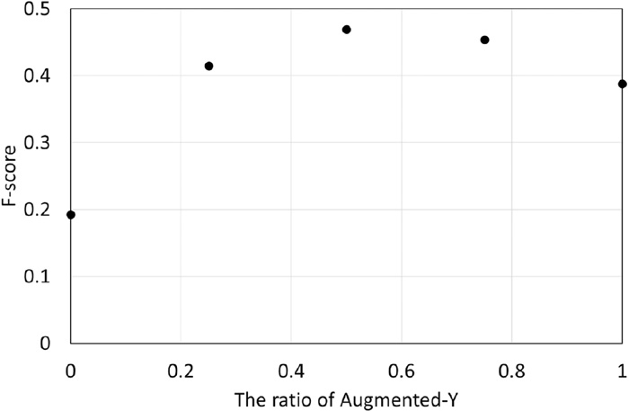
As shown in Fig. 4, the performance when 192 images of Augmented-S were used with the same number of images of Augmented-Y was not as good as when a smaller number of images of Augmented-S was used. This may be because the labeling in Augmented-S is less accurate than that in Augmented-Y. That is, assistance with Augmented-S may not be as good when the ratio of Augmented-Y becomes smaller. Different experimental conditions were prepared, as shown in #7 to #10 in Table 1. Those conditions and condition #1 have the same number of images in the training dataset with different ratios of Augmented-Y: 1, 0.75, 0.5, 0.25, and 0. The results for those conditions are shown in Fig. 5. As shown in Fig. 4, adding Augmented-S to Augmented-Y is effective in approximately half of the cases due to a lack of samples for thicker classes in Augmented-Y. Besides, there is an indication of a tendency in Fig. 4. A negative effect defeats a positive effect when the ratio of Augmented-Y becomes less than half. Here, the F-score of 0.5 in Fig. 5 was slightly higher than that for 192 of Augmented-S in Fig. 4. The former condition has half the number of images in the training dataset at the same ratio of Augmented-Y and Augmented-S: this is opposite to our expectation because models generally perform well with a larger number of images. This unexpected outcome may have originated from the similarity among the features of the images for the test dataset and 96 images that are randomly selected from 192 images of Augmented-Y.
While the PSPNet model was shown to perform effectively for the classification of thickness or diameter of steel contained in heavy steel scrap, we do not understand how the model recognizes the features of different classes in thickness or diameter. One of our expected features was the curvature and crumple of steel because of unintentional deformation during scrap processing. In the event that these characteristics dominate the recognition in the model, the scale of the images would not be sensitive to the performance. Therefore, in similar conditions to #6 in Table 1, the performance of our model was compared for three different sets of 192 images of Augmented-S. Those sets are prepared from Augmented-S-equ (#6), Augmented-S-5/6, and Augmented-S-5/9. As the results of learning with those datasets, the distribution of pixels predicted for the 3 - 6 mm class is shown in Fig. 6(a). In Fig. 6(a), the white three bars indicate True Positive for each condition. Despite the similarity of the portions of the True Positive in every scale of Augmented-S, the portions of the False Positive in the other two classes differed significantly for the scale of Augmented-S. The Augmented-S-5/9 has a larger length per pixel in the images in which steel of the same size looks smaller. The portion of the class predicted as less than 3 mm becomes larger according to the length per pixel in the images in those three conditions. The distribution of pixels predicted as 6 mm or more by the original class is shown in Fig. 6(b). In Fig. 6(b), the white three bars indicate True Positive for each condition but decrease according to the length per pixel in the images. The same tendency as Fig. 6(a) is found: the portion of the class predicted as less than 3 mm becomes larger. It was found that the classes of less than 3 mm and 6 mm or more are sensitive to the scale of images.
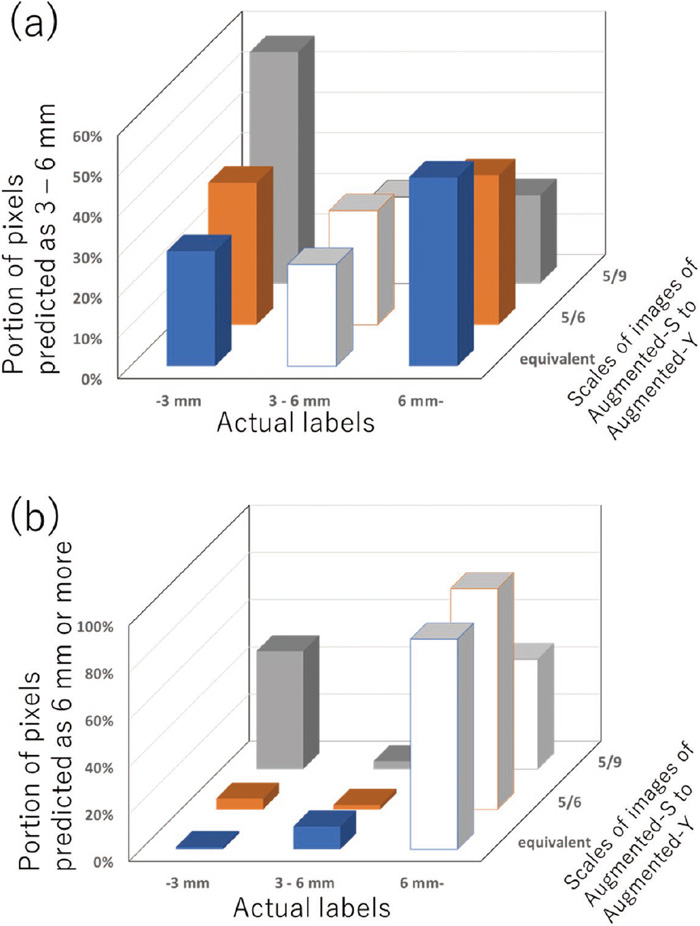
This result confirms that the developed model does not ignore the scale of images regardless of whether the cross-sectional area is observed. In the test images, the cross-sectional area can be observed for several steel units. The predicted class for those units of steel was true positive at the same portion as other steel units. We can conclude that the developed model relies mainly on the features related to deformation and refers to the scale of images.
5. Conclusions
This study was the first trial of employing a deep-learning-based image analysis technique to detect the thickness or diameter of steel without taking measurements. This trial revealed both the potential of using image analysis techniques on steel scrap and the problems involved. As a deep-learning-based image analysis, the semantic segmentation based on PSPNet was shown to effectively classify the thickness or diameter of steel in heavy steel scrap, even in the case of images in which the thickness or diameter in the cross-section of the steel cannot be observed. In our developed model, by compiling around 200 images with accurate ground-truth labeling and around 130 images with quasi-ground-truth labeling for the training dataset, the best F-score was almost 0.5 for the three classes of thickness or diameter less than 3 mm, 3 to 6 mm, and 6 mm or more. Notably, the F-score for the less than 3 mm class was more than 0.9. While the procedures for image acquisition and annotation were shown to perform well, there is much room for improvement in the resolution and input size of images and in labelling the classes. For the sake of empirical image acquisition, we ensure that the shortage of the number of images with accurate ground-truth labels can be complemented by the images with labeling based on the grades of steel scrap judged in the market as quasi-ground-truth labels. We believe that our developed model relies mainly on the features of deformation. While the developed model does not observe the cross-section of steel to predict the thickness, the experimental results show that the model refers to the scale of images. Therefore, the scale of images should be constant in the preparation of images.
Acknowledgement
This project is partially supported by New Energy and Industrial Technology Development Organization (Innovative Structural Materials Association and Entrepreneurs Program JPNP14012). The authors also acknowledge Bright Innovation Co., Ltd., ECONECOL Inc., and MM&KENZAI Corporation for their assistance in acquiring image data.
References
- 1) I. Daigo, S. Koketsu, P. Dunuwila and T. Hoshino: Dev. Eng., 25 (2019), 63 (in Japanese).
- 2) I. Daigo, K. Tajima, H. Hayashi, D. Panasiuk, K. Takeyama, H. Ono, Y. Kobayashi, K. Nakajima and T. Hoshino: ISIJ Int., 61 (2021), 498. https://doi.org/10.2355/isijinternational.ISIJINT-2020-377
- 3) I. Daigo, D. Fujimaki, Y. Matsuno and Y. Adachi: Tetsu-to-Hagané, 91 (2005), 171 (in Japanese). https://doi.org/10.2355/tetsutohagane1955.91.1_171
- 4) K. E. Daehn, A. Cabrera Serrenho and J. M. Allwood: Environ. Sci. Technol., 51 (2017), 6599. https://doi.org/10.1021/acs.est.7b00997
- 5) I. Daigo, S. Koketsu, S. Ota, H. Hayashi and M. Enoki: Tetsu-to-Hagané, 104 (2018), 461 (in Japanese). https://doi.org/10.2355/tetsutohagane.TETSU-2018-009
- 6) I. Daigo and Y. Goto: ISIJ Int., 55 (2015), 2027. https://doi.org/10.2355/isijinternational.ISIJINT-2015-166
- 7) D. Panasiuk, I. Daigo, T. Hoshino, H. Hayashi, E. Yamasue, T. D. Huy, B. Sprecher, F. Shi and V. Shatokha: J. Ind. Ecol., 26 (2022), 1040. https://doi.org/10.1111/jiec.13246
- 8) I. Daigo, L. Fujimura, H. Hayashi, E. Yamasue, S. Ohta, T. D. Huy and Y. Goto: ISIJ Int., 57 (2017), 388. https://doi.org/10.2355/isijinternational.ISIJINT-2016-500
- 9) A. Javaid and E. Essadiqi: Final Report on Scrap Management, Sorting and Classification of Steel, 2003-23(CF), Government of Canada, Ottawa, (2003), 19.
- 10) M. Robalinho and P. Fernandes: Proc. 16th Int. Conf. on Informatics in Control, Automation and Robotics (ICINCO 2019), Vol. 2, SciTePress, Setúbal, (2019), 666.
- 11) G. Seko and M. Nagata: Inspection Method and System for Steel Scrap, Japan Patent 2020-176909A, (2020) (in Japanese).
- 12) T. Wieczorek and M. Pilarczyk: Arch. Metall. Mater., 53 (2008), 613.
- 13) The Japan Ferrous Raw Materials Association: Year Book of Ferrous Raw Materials, Vol. 16, The Japan Ferrous Raw Materials Association, Tokyo, (2008), 121 (in Japanese).
- 14) W. Zhuo, M. Salzmann, X. He and M. Liu: 2017 IEEE Conf. on Computer Vision and Pattern Recognition (CVPR), (2017), 6269. https://doi.org/10.1109/CVPR.2017.664
- 15) J. Lazarow, K. Lee, K. Shi and Z. Tu: 2020 IEEE/CVF Conf. on Computer Vision and Pattern Recognition (CVPR), (2020), 10717. https://doi.org/10.1109/CVPR42600.2020.01073
- 16) H. Zhao, J. Shi, X. Qi, X. Wang and J. Jia: 2017 IEEE Conf. on Computer Vision and Pattern Recognition (CVPR), (2017), 2881. https://doi.org/10.48550/arXiv.1612.01105
- 17) E. Shelhamer, J. Long and T. Darrell: IEEE Trans. Pattern Anal. Mach. Intell., 39 (2017), 640. https://doi.org/10.1109/TPAMI.2016.2572683
- 18) B. Zhou, H. Zhao, X. Puig, S. Fidler, A. Barriuso and A. Torralba: 2017 IEEE Conf. on Computer Vision and Pattern Recognition (CVPR), (2017), 5122. https://doi.org/10.1109/CVPR.2017.544
- 19) B. Zhou, H. Zhao, X. Puig, T. Xiao, S. Fidler, A. Barriuso and A. Torralba: Int. J. Comput. Vis., 127 (2019), 302. https://doi.org/10.1007/s11263-018-1140-0
- 20) SuperAnnotate: Website of SuperAnnotate, https://www.superannotate.com/, (accessed 2022-05-15).
- 21) H. S. Munawar, F. Ullah, D. Shahzad, A. Heravi, S. Qayyum and J. Akram: Buildings, 12 (2022), 156. https://doi.org/10.3390/buildings12020156
- 22) C. D. Manning, P. Raghavan and H. Schütze: Introduction to Information Retrieval, Cambridge University Press, Cambridge, UK, (2008), 544.
