Regular Article
A Shallow Neural Network for Recognition of Strip Steel Surface Defects Based on Attention Mechanism
2023 Volume 63 Issue 3 Pages 525-533

Details
2023 Volume 63 Issue 3 Pages 525-533
This research proposes an efficient strip steel surface defect classification model (ASNet) based on convolutional neural network (CNN), which can run in real time on commonly used serial computing platforms. We only used a very shallow CNN structure to extract features of the defect images, and an attention layer which makes the model ignore some irrelevant noise and obtain an effective description of the defects is designed. In addition, a nonlinear perceptron is added to the top of the model to recognize defects based on the extracted features. On the strip steel surface defect image dataset NEU-CLS, our model achieves an average classification accuracy of 99.9%, while the number of parameters of the model is only 0.041 M and the computational complexity of the model is 98.1 M FLOPs. It can meet the requirements of real-time operation and large-scale deployment on a common serial computing platform with high recognition accuracy.
Defects on strip steel surface can affect the appearance of the strip steel, some defects even have a serious damage to the quality of the product. Therefore, the classification of the strip surface defects is one of the important bases for the inspection of the strip steel product quality. Compared with the traditional manual quality inspection, defect detection by computer vision methods has the advantages of high inspection efficiency, noncontact and non-destructive detection, and it is gradually applied to the inspection of industrial products.1,2)
In general, image classification task can be solved by pattern recognition methods, for example Support Vector Machines3) (SVM), Naive Bayes,4) Decision Tree,5) Perceptron6) etc. Manual selection of features is required when using pattern recognition methods to classify defect images, however, the surface images of strip steel are easily affected by light, material changes, oil stains, and many other noises. Besides, the image grayscale distribution of the same defect on the strip steel surface is wide, furthermore, there are many similarities between different types of strip steel defects.7)
Therefore, it requires careful tuning of model parameters and selection of reasonable features to obtain satisfactory accuracy with pattern recognition methods. The approach that utilizes deep learning methods for image classification has rapidly gained popularity in recent years. Compared to the manual feature selection in pattern recognition methods, deep learning based visual recognition models typically use multilayer convolution for automatic feature selection8) and are able to adaptively change the feature extraction methods in end-to-end iterative optimization.
For the task of image classification, deep learning based methods have shown excellent ability, many network structures with excellent performance have been proposed one after another, such as AlexNet,9) VGG,10) GoogleNet,11) ResNets12,13) which are used as backbone networks in numerous deep learning models, and EfficientNet.14) Deep learning based models perform far better than pattern recognition methods with manual features selection in complex computer vision classification task.15)
In some studies, strip defect classification has been performed on the basis of CNN models. Fu et al. utilize SqueezeNet16) as the backbone network, an additional multi-receptive field module was added to construct a strip steel defect recognition model, it can accurately classify defects while running in real time on a normal GPU.17) Wang et al. constructed a defect classification model that can run on GPU in real time by shrinking the fully connected layer structure of the original VGG network to reduce the number of parameters of raw model.18) Some methods first increase the volume of the strip steel defect dataset based on generative adversarial networks19) (GAN) and then construct CNN model for classification,20,21) which also achieved high classification accuracy. In addition to convolutional neural networks, ViT22) (Vision Transformer) based method has also been studied,23) but the classification accuracy achieved is lower in comparison with the CNN based methods. However, the existing CNN-based strip steel surface defect classification models have a large number of parameters as well as high computational cost, which is not suitable for real-time operation on serial computing platforms with limited computing power. In addition, some pattern recognition methods with manual feature selection have also achieved promising classification accuracy when classifying strip steel surface defects. Such as the benchmark experiment in24) which used six features from Grey Level Co-occurrence Matrix (GLCM) combined with support vector machine to recognize strip steel surface defects and achieved a promising accuracy of 90.81%. Therefore, the background and image structure of strip steel surface defect images are very simple compared with complex classification task.15) So, the features required to classify strip steel surface defects do not need to be very complex, a reasonably designed shallow CNN model can classify strip steel surface defects efficiently and accurately.
In order to extract the features of strip steel surface defects and design a classification model that can be executed in real time on a low-power serial computing platform, in this paper, we design a strip steel surface defect classification model with simple network structure, small number of parameters and high real-time computing capability, and name it ASNet (Shallow Neural network with Attention). For image feature extraction, the model uses a convolutional layer stacking approach similar to VGG.10) In addition, due to the simple structure of the strip steel defect images, we adopt an attention mechanism that allows the model to ignore part of information which is not related to the defects and focus on the defects itself, which augments the ability of the model to extract more effective defect features. At last, the extracted defect features are classified by a multilayer nonlinear perceptron. We evaluated the performance of our model on the NEU-CLS25) dataset, and the experimental results show that our model is able to run in real-time on a low-power serial computing platform, while being able to recognize strip steel surface defects very accurately.
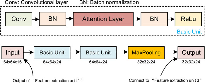
The overall network structure is shown in Fig. 1, which is composed of four feature extraction units, and a nonlinear perceptron. The spatial size and dimension of the feature map and the dimension of the feature vector for each part are given on the right side of Fig. 1. The “feature extraction unit 1”, “feature extraction unit 3”, and “feature extraction unit 4” have the same structure. In comparison with these three feature extraction units, “feature extraction unit 2” contains an additional attention layer, which is used to extract defective features more efficiently. The structure of the feature extraction unit is described in Section 2.2, and the “attention layer” is described in Section 2.3.

The overall network structure of our model. (Online version in color.)
The structure of the feature extraction unit is shown in Fig. 2. As can be seen, there are two stacked convolutional layers, and the function of these two stacked convolutional layers is to further extract features from the original image or feature map, where size denotes the spatial size of the convolutional kernels used in the convolutional layer. According to VGG,10) the size of the convolutional kernels used in all feature extraction units is 3 × 3. In addition, the convolutional layer of each feature extraction unit is followed by a batch normalization26) (BN) layer and a ReLu nonlinear activation function, which are used to augment the stability of the model during training and the nonlinear expression ability of the model, respectively.

The structure of feature extraction unit. (Online version in color.)
In addition, in order to reduce the memory usage, we perform down-sampling for the feature map from the feature extraction unit by maximum pooling to reduce the spatial size of the feature map to half of the original size.
2.3. Attention LayerThe convolution operation is spatially invariant, i.e., extracting defective image features with convolutional neural networks, the location of defective information in the feature map remains basically unchanged with respect to the overall feature map, even though the spatial size of the feature map decreases with increasing the number of convolutional layers. We take advantage of the characteristic to implement an attention layer for feature maps located at the shallow layer of the network, the role of the attention layer is to use the information provided by the feature map at the shallow location of the model to filter information that is not related to the defect. Ideally, the attention layer can retain the useful information related to the defect in the feature map, filter out the useless information (background, noise, etc.), reduce the flow of invalid information to the deeper convolutional layers, and make the feature map in the deeper layers of the network to describe the defect image more effectively.
The structure of the attention layer is shown in Fig. 3, the leftmost part of Fig. 3 shows the feature map output by the front convolutional layer (which is also the input feature map of the attention layer), and the rightmost part shows the output feature map of the attention layer. The symbol D denotes the feature dimension of the two feature maps, and W, H denotes the width and height of the feature maps respectively (the input and output feature maps of the attention layer have the same size in each dimension). Then we introduce the initial stage computational process of the attention layer, which first takes out the features at different locations of the input feature map (in Fig. 3, position P is used as an example), then the picked feature is fed into a perceptron with input dimension D and output dimension C+1, where C is the number of categories in the classification task (the number of categories in this paper is 6, so the output of the perceptron in Fig. 3 is 7 dimensions), and the additional categories are treated as invalid information. The output of the perceptron is passed through the Softmax function (which is shown in Eq. (1), where xn indicates the value of the feature vector at position n.) as the confidence score describing the individual features. The second stage of the attention layer computation process is to generate the mask of the input feature map (“Attention Mask” in Fig. 3), which has the same width and height as the feature map input to the attention layer, but the values at each position are scalars. The process of calculating the values at each position of the mask is as follows: the previously generated confidence scores and the manually selected weighting factors are weighted and summed, and then the results are fed into the ReLu function (Which is shown in Eq. (2), where x represents the input of the function) to obtain the mask values. Once the previously mentioned mask is calculated, the output feature map of the attention layer is obtained by multiplying this mask with the input feature map by position.
| (1) |
| (2) |

The architecture of attention layer, where Input Feature map denotes the output of previous convolutional layer, Output Feature map denotes the output of attention layer. (Online version in color.)
We then describe the learning process of the attention layer. From the previous description, it is clear that the learnable parameters of the attention layer are all in the perceptron in the initial computation stage, but the C+1 dimensional confidence scores output by the perceptron are without true labels, i.e., the attention layer cannot update the weights of the perceptron directly based on the confidence scores predicted in the initial stage. However, the confidence scores predicted by the perceptron have an effect on the feature map output by the attention layer, the feature map is then propagated in the network so the weights of the attention layer are updated during the back-propagation of the network.
To better understand why the attention layer has the ability to filter out invalid information from the feature map, we further describe the role of the weighting factor and its generic selection method. From Fig. 3, it can be known that the weighting factor is a C+1 dimensional vector and contains a unique negative number which is used to weight the confidence score of the invalid information for attenuating the value of the “Attention Mask”. Which means that if the attention layer needs to attenuate the feature at a certain position of the feature map, it only needs to increase the confidence score corresponding to that negative position (e.g., in Fig. 3, the attention layer wants to attenuate the feature at position P, what the attention layer needs to do is increase the first dimension of the confidence scores), and the attention layer is fully capable of completely nullifying the feature (because the weighted results of the confidence scores is fed into the ReLu function), meanwhile the decision of the attention layer affects the probability value of the final prediction of the model, so it can improve its own discriminative ability during the back propagation of the model. The general selection method of the weighting factors can be referred to Eq. (3). In Eq. (3), c0 denotes the unique negative value mentioned above, c1,...,cn denotes the remaining C positive values in the weighting factor, which is used to maintain the features rather than attenuation. The number of positive weighting factors should equal to the number of defect classes, because we want to mimic the classification process, i.e., we want the attention layer to be able to roughly distinguish valid information belonging to different classes of defects while filtering out useless information. In Eq. (3) symbol p can be considered as a threshold, i.e., a feature is completely nulled when the confidence score of the invalid information of a single feature in the feature map is greater than p (the attention layer produces a mask with a value of 0 at that feature location). As for c1,...,cn, their values are generally all set to 1, because when these values are all set to 1, the attention layer produces a mask with a maximum value of 1, which can ensure that the values of the feature maps input to the attention layer will not be scaled up, and maintain the stability of the model values during training. Of course, if the number of defective images in each category in the training dataset is significantly unbalanced, the weighting factor can be changed, for example, by properly increasing or decreasing any of the values of c1,...,cn can give the attention layer a priori knowledge of the class imbalance and may improve the performance of the model. The dataset used in this paper has a balanced number of defects of all categories, and we do not want to add any a priori knowledge to the model, so the c1,...,cn are all set to 1, and the threshold p is set to 0.5 (We set p to 0.5, which equivalent to leaving the attention layer to independently decide whether the features at each position of the feature map is valid information, without introducing additional human considerations.), i.e., in this paper, the unique negative value in the weighting factor is −1.
| (3) |
The structure of the feature extraction unit which contains the attention layer is shown in Fig. 4, we chose to add the attention layer to the coarse feature maps, because the convolutional layer has not yet deeply fused the background and noise information with the effective information at this time. So, the attention layer is more likely to take out the valid information.
Structure of feature extraction unit which includes the attention layer. (Online version in color.)
For the classification, we adopt a three layers nonlinear perceptron. The number of nodes in the hidden layer of the perceptron is 16,32,16, and each node in the hidden layer is activated with the ReLu nonlinear function. The input feature of the perceptron is the feature vector obtained from the global pooling of the feature map output by the “feature extraction unit 4”. The number of nodes for the output layer of the perceptron is equal to the number of defect categories, and the output value of each node represents the probability (with Softmax activation function) that the feature vector input to the perceptron corresponds to different category of defects.
We evaluate our model with the NEU-CLS dataset, a dataset of surface defects of hot-rolled strip steel from Northeastern University, China. The dataset consists of six typical surface defects of hot rolled strip: crazing, inclusion, patches, pitted-surface, rolled-in-scale and scratches. Each category of defect images has 300 images with a raw resolution of 200 × 200. The appearance of each type of defect is shown in Fig. 5. As can be seen from Fig. 5, the grayscale distribution of different categories of defects is not uniform, and the geometric shape of different defects is also not uniform. Such as the two different defects of inclusions and scratches are flat, while the geometric distribution of patches is blocky, and the area of crazing and pitted-surface defects is small and randomly distributed throughout the image range. In addition, the grayscale distribution of the same defect in this dataset is also widely distributed.

Sample images of different categories of defects.
Considering that the setup of the vision system in practice may affect the image quality, we further extended the validation dataset. Line scan cameras are widely used in strip steel production lines to build vision acquisition systems, the characteristics of line scan cameras ensure that there is no motion blur in the acquired images. The vision system which is built with line scan cameras often requires careful adjustment of the position and angle of the bar light to ensure uniform image acquisition, therefore, the captured images are almost free from uneven illumination. However, the contrast of the images is affected by the bar light illumination intensity and the angle of the bar light, in addition, considering that there may be some noise in the captured images, we enhance the validation dataset from the following two ways.
Multiple contrast enhancement: We adopt Eq. (4) to adjust the contrast of images with different coefficients k, where x denotes the grayscale of pixels at different locations, avg denotes the mean of the grayscale of the image. Based on the number of images for training, we selected different number and value of coefficients k to enhance the validation dataset. The candidate coefficients are 0.8,1.2,1.4,1.6,1.8 and 2.0, which greatly enriches the contrast of the images in validation dataset.
| (4) |
Noise: Considering the characteristic of high accuracy of line scan camera, we only added small noise to the validation images, Gaussian noise with 35 signal-to-noise ratio (SNR) is added to the validation images. SNR is defined as
| (5) |

Sample of defect images in both the origin dataset (first row) and the enhanced validation dataset, which including contrast enhancement (second and third rows) and noise image (fourth row).
We implement our model with the Tensorflow deep learning framework. The experimental platform is: Intel Xeon Gold 6142 CPU@ 2.60GH processor, 28 GB RAM, NVIDIA GeForce RTX3080 graphics card, and the operating system is Ubuntu with version number 20.04. 80% of the total data is used as the training set and the remaining 20% as the validation set. Our model is trained using backpropagation27) by Adam.28) During the training process, the cosine decay schedule29) is adopted to adjust learning rate. We train the model for 300 epochs with batch size 128. We reduce the resolution of the image to 128 × 128 and augment the image of the training set by randomly flipping the image horizontally and vertically, slightly increasing or decreasing the contrast of the image.
For experiment, the number of filters of the convolutional layer of “feature extraction unit 1” is set to 16, the number of filters of the convolutional layer of “feature extraction unit 2” and “feature extraction unit 3” is set to 24, and the number of filters of the convolutional layer of “feature extraction unit 4” is set to 32, all convolutional layer parameters were initialized with the method introduced in.30)
3.4. Results and AnalysisWe evaluate the performance of our model with the following three performance metrics: computational complexity, classification accuracy, and inference efficiency. To match the actual hardware platform of our model more closely, the model will run on a mobile CPU with Intel Core i7-9750 H@ 2.6 GHz when evaluating the inference efficiency of our model.
Since our model has a very small number of parameters, low computational complexity, and the dataset used for experiments is not large, a training process takes only a short time. In order to evaluate the performance of our model more accurately, when evaluating the classification accuracy of the model, we use a program to generate some random number seeds, which are used to randomly partition the dataset, and train the model 40 times using the completely randomly partitioned data, and take the average accuracy of these 40 training sessions to evaluate the classification accuracy of our model. Furthermore, we also count the standard deviation of the classification accuracy of these 40 sessions to evaluate the stability of the classification accuracy of our model. The inference efficiency of our model is evaluated by running the model 12 times consecutively, each time with a different image input, counting the time consumed by the model for each inference, removing the maximum and minimum values, and taking the average running time to evaluate the inference efficiency of our model.
The performance of our model on the NEU-CLS dataset and the comparison results with some popular models are given in Table 1. From the results presented in Table 1, it can be seen that our model achieves higher classification accuracy than some popular models such as ResNet50, VGG16, DenseNet121, and the commonly used lightweight network MobileNetV3 (Large) in the classification of steel surface defects (We think the reason for the lower performance of these SOTA models is the insufficient amount of training data). Meanwhile the number of parameters and the computational cost of our model are significantly reduced compared to the models mentioned above. Compared with Mix-Fusion,24) a lightweight steel surface defect classification model, the classification accuracy of our model is improved by 1.3%, and the number of parameters is only 1/6 of Mix-Fusion, in addition, the standard deviation of the classification accuracy of our model on the validation set is only 0.16 in 40 training sessions on a random 8:2 divided dataset (Table 2), which shows that our model can keep good stability and obtaining high accuracy when classifying strip steel surface defects. In terms of inference efficiency, our model takes only 0.026 seconds to process an image without computational optimization when running on a low-power mobile CPU, i.e., it can process up to 38 images per second, allowing real-time classification of defects on commonly used serial computing platforms.
| Splitting (%) | Origin (%) | Contrast (%) | Noise (%) | Standard Deviation | ||
|---|---|---|---|---|---|---|
| Origin | Contrast | Noise | ||||
| 80 | 99.9 | 88.9 | 99.7 | 0.16 | 1.96 | 0.11 |
| 50 | 99.7 | 87.0 | 99.0 | 0.20 | 2.83 | 0.34 |
| 25 | 99.1 | 88.4 | 98.8 | 0.35 | 2.71 | 0.26 |
| 10 | 97.3 | 92.4 | 96.5 | 0.66 | 1.97 | 0.54 |
Due to the small amount of data contained in NEU-CLS, only 360 images were used for validation when 80% of the total data was used for training. In order to further investigate the ability of our model to extract effective defect features, we further train our model with different percentages of data to investigate the variation of classification accuracy. Table 2 (detailed explanation in Section 3.5) presents the classification accuracies obtained by training the model with different percentages of total data. The results are obtained by randomly dividing the total data into training and validation datasets with the currently configured percentage of training data, training the model 40 times, and presenting the average accuracy and the standard deviation of the accuracy on the validation dataset.
As shown in Table 2, our model achieves high classification accuracy with different proportions of data for training, and the standard deviation of the model classification accuracy increases slightly as the number of images used for training decreases, but remains in a stable state. When only 10% of total data is used for training and 90% for validation, our model still achieves an average classification accuracy of 97.3%, which is 11.7% higher compared to the lightweight classification network in24) when the same percentage of data is used for training. In addition, our model performance did not degrade rapidly when the amount of training data was reduced, so the model is able to filter out useless information during training process partly and obtain an effective description of defects. To describe the convergence properties of our model, the loss and accuracy variation curves during the training process are shown in Fig. 7, where the red and blue curves in Fig. 7(a) indicate the variation of the loss values on the training and validation sets, respectively, during the training process, and the red and blue curves in Fig. 7(b) indicate the variation of the accuracy of the model on the training and validation sets, respectively, during the training process.

Loss value(a.) and classification accuracy(b.) variation curves during training process. (Online version in color.)
As can be seen from Fig. 7, the accuracy and loss values of the model fluctuate drastically at the beginning of the training, the model performance is very unstable, however, as the number of iterations increases, the accuracy and loss values of the model become very stable. There are two possible reasons for this phenomenon: on the one hand, our model has a small number of parameters, the learning rate is large at the initial stage, so update the model weights once will make the whole model parameters to fluctuate, resulting in the model performance being affected. On the other hand, we implemented data augmentation, the model (especially for the attention layer) requires several iterations to deal with the spatial location and grayscale changes of the images in training set, extract the key information and classify the defects effectively. When we remove the data augmentation, the performance of our model is much more stable on the validation set in the initial stage, but with the data augmentation we can make a slight improvement of the performance of our model, so we keep the data augmentation in our experiments.
3.5. The Effects of the Attention LayerThe original motivation for proposing an attention layer in this paper is to make the model focus on the defects and ignore some background and noise information that are not relevant to the defects. Therefore, ideally, the attention layer will either attenuate or zero out the information in the feature map that is not related to the defect identification, and keep the local areas in the feature map that contain the defect information.
For a straightforward understanding on how the attention layer works, we visually present the mask of the attention layer in Fig. 8, where the selected defect images are shown in the first and third rows, and the output mask image of the attention layer is shown below them. As can be seen from the mask image in Fig. 8: the attention layer gives a high response at the location of the defect corresponding to the image, while the response is weak at some irrelevant background and noisy locations, so even without the defect-specific location labels (i.e., we do not label the exact location of the defect in the defect images), the attention layer is still able to recognize the key information in the end-to-end training, which meets our initial expectations in designing the attention layer.

Defect images (top) and the corresponding feature maps of the attention layer mask output (bottom). (Online version in color.)
In order to investigate the effects of the attention layer in our model, we remove the attention layer from the model, train the model without the attention layer, the full experimental results are shown in Tables 2 and 3. In Tables 2 and 3, the first column indicates the percentage of data used for training, the next three columns represent the accuracy obtained by the model on three different types of validation datasets respectively, and the last column indicates the standard deviation of the model accuracy. Here we further explain the three different validation datasets in details:
| Splitting (%) | Origin (%) | Contrast (%) | Noise (%) | Standard Deviation | ||
|---|---|---|---|---|---|---|
| Origin | Contrast | Noise | ||||
| 80 | 99.8 | 87.0 | 99.0 | 0.27 | 2.90 | 0.55 |
| 50 | 99.5 | 80.3 | 98.4 | 0.26 | 1.78 | 0.47 |
| 25 | 98.8 | 83.7 | 97.9 | 0.65 | 2.92 | 0.50 |
| 10 | 96.4 | 89.9 | 96.2 | 1.16 | 1.94 | 0.72 |
Origin: Using data from the original dataset for experiments, the two models (with attention layer and without attention layer) are trained exactly as described in Section 3.4.
Contrast: The original NEU-CLS dataset is randomly partitioned (based on the percentage of data for training), using the training dataset for models training, the data in the validation set is enhanced according to the contrast augmentation described in Section 3.2. When using 20% of the data for validation, we select all the contrast augmentation coefficients introduced in Section 3.2 to enhance the validation set, resulting in a total of 2160 validation images, when using 50% of the data for training, three contrast augmentation coefficients are selected (1.2,1.6 and 2.0) to enhance the validation set, resulting in a total of 2700 validation images, when using 25% of the data for training, two contrast augmentation coefficients are selected (0.8 and 1.4), resulting in a total of 2700 validation images, and when using 10% of the data for training, we choose one contrast enhancement factor (1.2) resulting in a total of 1620 validation images. It is worth noting that we discard the images in the original validation set and keep only the enhanced images for validation.
Noise: The data in the validation set is polluted by Gaussian noise with SNR of 35 db.
As can be seen from Tables 2 and 3, the performance of the model with the attention layer is better (Table 2) than that of the model without the attention layer (Table 3), both on the original validation dataset and the enhanced validation dataset. When only 10% of the data is used for training, the recognition accuracy of the model with the attention layer is 0.9% higher than that of the model without the attention layer. In particular, when the data in the validation set is enhanced with contrast, the recognition accuracy of the model with the attention layer is on average 4% higher than that of the model without the attention layer. Meanwhile, the standard deviation of model accuracy shows that the model with the attention layer is more stable in multiple training (when the validation set is enhanced, we train the two models 10 times repeatedly and report the accuracy and standard deviation).
Therefore, the extra attention layer can effectively deal with the problem of insufficient training data, and at the same time, the stability of the model performance can be further improved because the attention layer allows the model to filter out some useless information and focus on the defects. Meanwhile, the attention layer only introduces less than 500 parameters, while complexity of the computational process is low, therefore the addition of the attention layer is with almost no effect on the inference efficiency of the model.
In order to verify the effectiveness of the additional design in our model, we remove the additional parts of the model, leaving only the stacking approach exactly the same as the VGG network structure, and use it as the baseline model. The number of parameters in the baseline model is 0.04 M, which is comparable to our model, so the effect of the reduced number of parameters on the performance of the baseline model can be ignored.
We train the baseline model with the approach introduced in Sections 3.3 and 3.4, using half of the dataset as the training set and the other half as the validation set. We counted the classification accuracies on each training as a scatter plot in Fig. 9, where the horizontal axis of Fig. 9 indicates the order of training and its vertical axis indicates the accuracy obtained on the validation set for that training. As can be seen from Fig. 9, the accuracy of the baseline model fluctuates obviously in 40 training sessions, so the baseline model is vulnerable to the training data and the initial parameters of the model. We further calculated the average accuracy of the baseline model for 40 training sessions, which is 98.4% with a standard deviation of 1.06. Compared with our model, the accuracy is reduced by 1.3% and the standard deviation is increased by 0.86.

Accuracy distribution of the baseline model for 40 training process. (Online version in color.)
Comparing the baseline model with our model, our model is obviously better than the baseline model in terms of convergence performance, classification accuracy, data dependence and model stability, which fully demonstrates the effectiveness of the additional design of our model.
Considering the simple structure of the strip steel surface image, we introduced an attention layer and integrated it into a shallow convolutional neural network to construct a low-complexity model that can accurately recognize strip surface defects. The introduced attention layer has almost no impact on the model size and efficiency, while noticeably increasing the recognition accuracy and stability of the model. Furthermore, the low computational complexity of our model also allows the model to run in real time on the commonly used serial computing platforms, making it suitable for large-scale deployments. Although the network training is initially unstable, but it can be stabilized by increasing the number of training iterations and reasonably adjusting the learning rate.
This work was supported by the Natural Science Foundation of Anhui Province under Grant No. 2108085MF225.