Regular Article
A Mixing Model Using Scale Factors for Prediction of Intermixed Bloom Concentration of 0.4mass%C-0.2mass%Si-0.7mass%Mn Steel in Continuous Casting

2023 Volume 63 Issue 3 Pages 504-515
Details
2023 Volume 63 Issue 3 Pages 504-515
Although there have been studies on models for predicting the mixing concentration of elements between old and new molten steel with different chemical components during continuous casting, there is limited information about the concentration of the mixed portion in the cross-sectional and the longitudinal directions of the intermixed bloom. In the present study, the concentration of the intermixed bloom generated by the different-grade continuous casting is measured in the cross-sectional and the longitudinal directions. A significant difference in the concentration of the mixed portion is noticed at different heights along the thickness direction of the intermixed bloom. Based on the measurement results, we propose a new mixing prediction model that can accurately predict the concentration of the mixed portion at the subsurface and the center in the intermixed bloom along the longitudinal direction. The present results show that each height which has the minimum and the maximum concentrations of the mixed portion in the cross-section varies along the longitudinal direction of the intermixed bloom. This implies that the maximum and the minimum concentrations of the mixed portion in the cross-section do not necessarily occur only at the surface and the center of the intermixed bloom. The newly proposed mixing prediction model can be employed to cut off the mixed portion by predicting the minimum and maximum concentrations of the mixed portion in the cross-section along the length direction of the intermixed bloom.
Different-grade continuous casting is one of the operating methods for improving the efficiency, flexibility, and productivity of continuous casting machines. However, the supply of new molten steel injected into the tundish generates a transition region that gradually changes the concentration of old molten steel remaining in the tundish. Therefore, it is necessary to accurately predict the mixed portion in the transition region and consequently, ensure their suitability for the steel grade.
In the present study, the term “strand” refers to a solidifying shell containing liquid molten steel, “bloom” refers to the final as-cast steel product that has been fully solidified and cut into pieces at the torch cut-off point,1) and the “intermixed bloom” refers to the bloom containing the mixed portion.
Figure 1 shows two representative methods for different-grade continuous casting using the same tundish. The “less mixing casting” (hereinafter, referred to as “LMC”) method is applied when there is a large concentration difference between old molten steel and new molten steel which have different concentrations of one or more chemical components. Meanwhile, the “mixing casting” (hereinafter, referred to as “MC”) method is applied when there is a relatively small concentration difference between two different grades of molten steel.
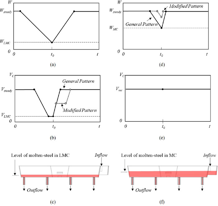
Methods for different-grade continuous casting using the same tundish. (a) Tundish weight as a function of time, (b) casting speed as a function of time, and (c) schematic of less mixing casting (LMC) at t=t0. (d) Tundish weight as a function of time, (e) casting speed as a function of time, and (f) schematic of mixing casting (MC) at t=t0. Wsteady, WLMC, t0, Vsteady, and VLMC refer to the steady state tundish weight, starting tundish weight of LMC, starting mixing time in the tundish, steady state casting speed, and starting casting speed of LMC, respectively. (Online version in color.)
In Figs. 1(a)–1(c), an LMC method is used for injecting new molten steel into the tundish by changing the casting speed. As shown in Fig. 1(a), the amount of remaining old molten steel in the tundish should be small as possible in order to reduce the mixed portion when the supply of new molten steel into the tundish starts at t = t0. Figure 1(b) shows the changes in the casting speed with time. The supply of molten steel injected into the mold should be continuous, and the casting speed should be gradually reduced. When new molten steel is supplied to the tundish, the casting speed is gradually increased by the time it reaches a desired casting speed of steady-state. With a gradually increasing casting speed, one or more holding sections with the same casting speed can be kept as the modified pattern of the casting speed shown in Fig. 1(b). Figure 1(c) shows the amount of remaining old molten steel in the tundish with the supply of new molten steel.
In Figs. 1(d)–1(f), an MC method is used to inject new molten steel into the tundish without changing the casting speed. As mentioned above, the amount of remaining old molten steel in the tundish must be minimized in order to reduce the amount of the mixed portion in the tundish. However, injected new molten steel into the tundish through a shroud nozzle is exposed to the atmosphere when the surface position of the remaining old molten steel in the tundish is lower than the tip position of the shroud nozzle, and a part of the exposed new molten steel is oxidized. Oxidized molten steel deteriorates the cleanliness of mixed molten steel in the tundish. To guarantee the cleanliness of mixed molten steel, new molten steel is injected into the tundish within the acceptable range of the amount of old molten steel when the surface position of the remaining old molten steel is higher than the tip position of the shroud nozzle. When the concentrations of old molten steel and new molten steel are similar to each other or have minimal differences, the amount of remaining old molten steel in the tundish is not artificially reduced to the modified pattern of the tundish weight shown in Fig. 1(d). The modified pattern of the tundish weight shown in Fig. 1(d) is the same as the general pattern of the tundish weight in the same grade continuous casting.
The intermixed blooms produced by the LMC method and by the MC method are scrapped and downgraded, respectively. It is important to develop a mixing prediction model that can accurately predict the mixed portion even if there are various operating methods such as the LMC and the MC methods in different-grade continuous casting according to changes in the tundish weight and the casting speed. Therefore, it is necessary to measure and accurately predict the concentration of the mixed portion produced by different-grade continuous casting.
Several studies1,2,3,4,5,6,7,8,9,10,11,12,13,14,15,16,17) have developed models to predict the concentration of the mixed portion during different-grade continuous casting. Huang and Thomas1) developed a three-dimensional mathematical model for predicting concentration profiles of the final slab in different-grade continuous casting, and reported reasonable agreement between predicted and experimental concentration profiles in the slab centerlines. Huang and Thomas2) proposed a mixing box model based on “tank in series” or “volumes” mathematical models consisting of three parameters, plug flow volume, mixing volume, and dead volume, which have been used to characterize steady flow in the arbitrary tundish configurations. The mixing box model divides each volume into two components to account for the effect of transient flow in the tundish and the strand, respectively, and calculates the composition distribution in the final slabs. Thereby, they developed the mixing prediction model, MIX1D code, which consists of three submodels with eight parameters related to the geometry of the systems such as the tundish and the mold, and verified the calculated results using the measured concentration of the mixed portion in the transition region. The MIX1D code was reported to be more efficient than Huang and Thomas’s previous model.1) However, several experimental data were additionally required to tune the eight parameters in order to increase the accuracy of the calculated results.
Goldschmit et al.3) extended the concept of “tank in series” or “volumes” mathematical models used in a single-line slab or symmetric two-line slab casting machines to be used in a symmetric four-line billet casting machine as well. The proposed mixing model distinguishes four lines of the billet caster into a group of two inner lines and the other group of two outer lines, and calculates individually the concentrations of the mixed portion in each group, respectively. The mixing model consists of three submodels, a tundish mixing model, a mold mixing model, and a final composition model, related to the geometry of the systems such as the tundish and the mold. The first submodel, the tundish mixing model, has nine parameters with four mixing volumes, two dead volumes, two plug flow volumes associated with two groups, and one extra recirculating mixing volume which allows mass flow between both groups. The second submodel, the mold mixing model, has six parameters with two mixing volumes, two plug flow volumes, and two convection-diffusion regions in both groups. The third submodel, the final composition model, solves the convection-diffusion equation using the turbulent diffusivity given by a 3D numerical model. The predicted concentration of the mixed portion by the mixing model was found to agree well with the measured concentration of the mixed portion in each group of the inner lines and the outer lines. The mixing prediction model was implemented in the GRADE code and applied to industrial problems. However, several parameters used in the mixing prediction model such as the model proposed by Huang and Thomas2) should be determined and modified through numerical and experimental results prior to the application of the model.
Cho and Kim4) proposed a simple tundish mixing model that calculates the concentration of the mixed portion using one scale factor related to the tundish configuration. The scale factor is the parameter that affects two weighting factors, and the sum of two weighting factors is one. The concentration of molten steel flowing out from the tundish was determined by the product of one weighting factor and the concentration of new steel flowing into the tundish, and the product of the other weighting factor and the average concentration of residual molten steel in the tundish. The previous mixing prediction models2,3) developed based on the “tank in series” or “volumes” mathematical models require the introduction of several parameters, but the mixing prediction model proposed by Cho and Kim4) has the advantage that it requires only one scale factor associated with the tundish configuration in obtaining the concentration of molten steel flowing out from the tundish. Therefore, their mixing prediction model is more practical than the other previous mixing prediction models.2,3)
Cho and Kim5) introduced an additional scale factor associated with the concentration of molten steel flowing out from the mold, extending the simple tundish mixing model4) to the strand region. Cho and Kim5) reported a small difference in the concentration of the mixed portion in the cross-section of the intermixed zone. The predicted concentrations of the mixed portion in the thin slab were consistent with the measured values. However, there are limited data on the measured concentration of the mixed portion in the intermixed zone of the bloom and the slab in their study.5)
In the present study, the concentration profiles of the mixed portion along the thickness and the length directions in the bloom with large-sized cross-sections have been measured. Through the measured results, it is found that the concentration difference between the center and the subsurface of the mixed portion is very large. It is found that, as the thickness of the cast steel is increased, the movement of molten steel to the center of the strand and diffusion in the mold by turbulent flow may be increased the concentration difference between the center and the subsurface of the mixed portion. Based on the measured results, a new mixing prediction model using two scale factors is proposed to predict individually the concentrations of the mixed portion at the center and the subsurface in bloom caster with multiple strands. The new mixing prediction model can minimize the number of parameters that should be tuned even if it is applied to multiple lines of the large sized bloom caster.
The present study is focused on the concentration prediction of the mixed portion in different-grade continuous casting in a curved bloom caster composed of one ladle, two tundishes, and eight molds, as shown in Fig. 2. Two tundishes of ‘h’-shape are arranged symmetrically facing each other. Molten steel in one tundish is distributed to four lines through a dam installed in the center of the tundish. Due to the properly designed shape of the dam, molten steel is symmetrically supplied to the molds through the dam.

Schematic of the continuous caster system used in the present study. (Online version in color.)
In a bloom caster with multiple strands, it is necessary to individually predict the concentration of the mixed portions generated in each strand according to operating conditions. Table 1 shows the approximate operation conditions for the LMC method. Figure 3 presents an intermixed bloom expected to be a mixed portion produced under the operating conditions listed in Table 1. As shown in Fig. 3(a), the locations of the head and the tail of the intermixed bloom are set to zero and 12 m in the length direction, respectively. The long 12 m intermixed bloom was cut into lengths of 7 and 5 m by the torch-cutting machine of the bloom caster. Figures 3(b) and 3(c) show the samples obtained from zones A and C, and zone B, respectively. In zones A and C, long samples were obtained in the thickness direction after cutting at intervals of 1 m, whereas the samples in zone B, including the subsurface and the center, were collected after cutting at intervals of 0.5 m.
| Steady-state tundish weight, Wsteady | Tundish weight in the starting state of LMC, WLMC | Steady-state casting speed, Vsteady | Casting speed in the starting state of LMC, VLMC | Pattern of the casting speed |
|---|---|---|---|---|
| 50 tons | 8.26 tons | 0.5 m/min | 0.1 m/min | Modified |
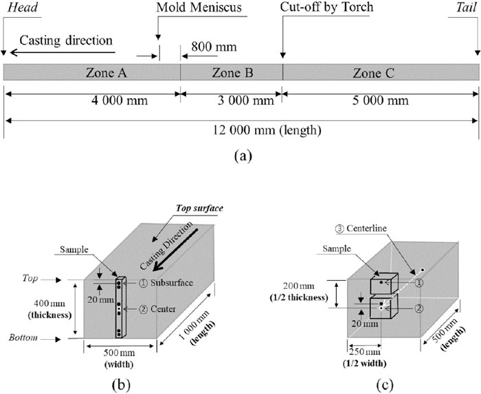
Information of the samples: (a) intermixed blooms, (b) sample in zone A and zone C, and (c) sample in zone B.
It was assumed that there was no difference in the concentration of the mixed portion in the thickness direction and that the concentration of the mixed portion changed rapidly in the length direction. Therefore, only the samples including the off-center and the subsurface of the intermixed bloom were taken at shorter intervals in zone B. After checking the results of the measured concentration of the sample in zone B, long samples were taken in the thickness direction from zones A and C.
The concentration of each element is analyzed and can be converted to a dimensionless concentration C(x,y,z) as follows:
| (1) |
Table 2 shows the chemical composition measured in old and new molten steel and the allowable range of concentration of each element in the old and new steel grades. Among the elements of the two steel grades, the difference in the concentration of chromium between old and new molten steel is the largest. Table 3 shows values obtained by converting the listed values in Table 2 into dimensionless concentrations using Eq. (1). The non-allowable range of dimensionless concentration of chromium that does not belong to any steel grades is 0.0722 to 0.9485. Among the elements, chromium has the largest non-allowable range of dimensionless concentration in chemical composition of molten steel investigated.
| C | Si | Mn | Cr | |
|---|---|---|---|---|
| Old molten steel (allowable range) | 0.413 (0.39–0.43) | 0.218 (0.15–0.25) | 0.746 (0.65–0.80) | 1.020 (0.95–1.10) |
| New molten steel (allowable range) | 0.380 (0.35–0.39) | 0.202 (0.15–0.25) | 0.563 (0.50–0.60) | 0.050 (~0.10) |
| C | Si | Mn | Cr | |
|---|---|---|---|---|
| Old molten steel (allowable range) | 0 (~0.6970) | 0 (all) | 0 (~0.5246) | 0 (~0.0722) |
| New molten steel (allowable range) | 1 (0.6970~) | 1 (all) | 1 (0.7978~) | 1 (0.9485~) |
Molten steel composition influences the segregation behavior of solute elements with low solubility or high content during solidification from the surface of the strand in the same grade continuous casting. Huang and Thomas1) reported that different elements should be affected equally by turbulence because the molecular diffusivity of elements is at least three orders of magnitude smaller than the turbulent diffusivity in molten steel. Huang and Thomas2) reported that the dimensionless concept is useful because most elements have been found to intermix equally except for carbon and aluminum which diffuse rapidly in the solid. Therefore, instead of carbon and manganese which have low solubility or diffuse rapidly in the solid, chromium with high content is selected as a representative value of the composition because of the largest concentration difference between the two steel grades and the largest non-allowable range of dimensionless concentration.
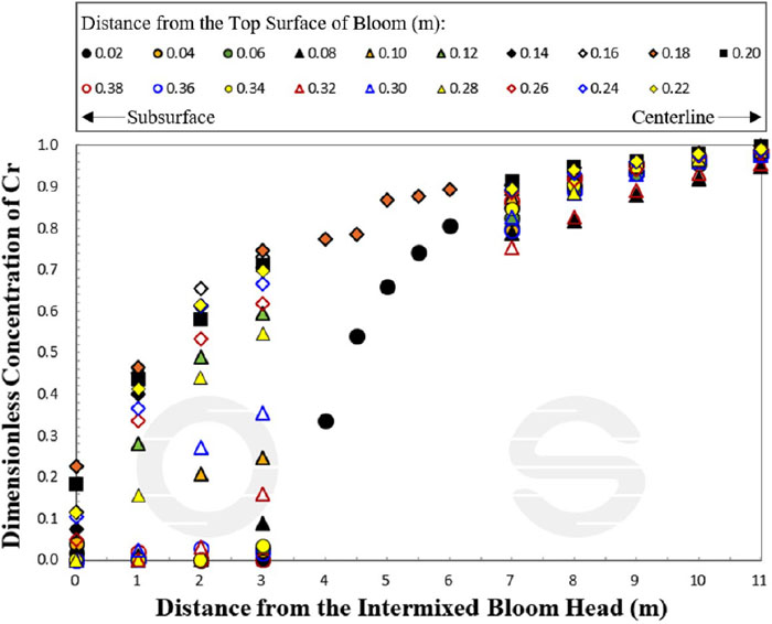
Figure 4 shows the conversion of the measured chromium concentration into a dimensionless concentration by Eq. (1) along the thickness direction at each longitudinal position of the intermixed bloom. At the zero position in the longitudinal direction (the head of the intermixed bloom), the equivalent dimensionless concentration of old molten steel is noted from 0.02 m (subsurface below the top surface) to 0.12 m (approximately 1/4 of the thickness) along the thickness direction. The dimensionless concentration of chromium is increased from 0.14 to 0.18 m (off-center, approximately 1/2 of the thickness), and is decreased from 0.20 m (center) to 0.28 m (approximately 3/4 of the thickness). Moreover, the equivalent dimensionless concentration of old molten steel is observed at the distance of 0.28 to 0.38 m (subsurface above the bottom surface) from the top surface as shown in Fig. 3(b).

Distribution of the measured concentration of chromium along the intermixed bloom of the first strand (WLMC = 8.26 ton, VLMC = 0.1 m/min). Symbols refer to the distance (m) from the head of the intermixed bloom. (Online version in color.)
At 1 m from the head of the intermixed bloom shown Fig. 3(a), the dimensionless concentration of old molten steel is observed at 0.02–0.10 m. The dimensionless concentration of chromium is significantly increased at the top surface position of 0.12–0.18 m. At 1–3 m from the head of the intermixed bloom, the dimensionless concentration of chromium starts to increase at closer distances to the top surface as further from the head of the intermixed bloom. At 4–11 m from the head of the intermixed bloom, the dimensionless concentration of chromium at the subsurface below the top surface starts to increase. At 11 m from the intermixed bloom head, a similar dimensionless concentration of new molten steel is noted throughout the thickness direction. At most longitudinal positions, the dimensionless concentration of chromium is larger at 0.18 m (off-center) than that at 0.2 m (center) in the thickness direction. In addition, the distribution of the dimensionless concentration of chromium in the thickness direction toward the tail of the intermixed bloom follows a W-shape.
Figure 5 shows the result of converting the x-axis of the data shown in Fig. 4 from the thickness direction to the length direction, and shows the dimensionless concentration of chromium along the length direction at each thickness point. The minimum dimensionless concentration of chromium at 7 to 11 m in the longitudinal direction is noted at 0.08 m (approximately 1/4 of the thickness) and 0.32 m (approximately 3/4 of the thickness) in the thickness direction. These results imply the need for a mixing model that predicts the maximum and the minimum dimensionless concentrations of the mixed portion in the cross-section. In other words, unlike the previous mixing models1,2,3,4,5) that predict the concentrations of the mixed portion at the surface and/or the centerline only, a mixing model for predicting the maximum and the minimum concentrations of the mixed portion in the cross-section can be more useful in removing the mixed portion.
Distribution of the measured concentration of chromium along the length direction of the first strand (WLMC = 8.26 ton, VLMC = 0.1 m/min). Symbols indicate the position (m) from the top surface. (Online version in color.)
Figure 6 shows the dimensionless concentrations of chromium along the length direction in the subsurface below the top surface, the subsurface above the bottom surface, and the off-center. The changes in the dimensionless concentration of chromium in each thickness point along the longitudinal direction follow a logarithmic function form. In addition, the gradient of the dimensionless concentration of chromium to the distance between two adjacent points in the longitudinal direction at the top subsurface and the bottom subsurface is larger than that at the off-center. Nevertheless, at the same longitudinal position, the dimensionless concentration of chromium at the off-center is always greater than that at the subsurface because the starting position for the increment of the dimensionless concentration of chromium at the off-center occurs before that at the subsurface. Jeong et al.6) reported a vortex structure through numerical analysis, in which the concentration of new molten steel propagates to the surrounding concentration of old molten steel while rapidly moving from the mold wall to the center of the strand in different-grade continuous casting. This phenomenon is attributed to the movement and diffusion of molten steel to the center of the strand due to the turbulent flow of molten steel in the mold. Molten steel injected into the mold through the submerged entry nozzle (SEN) strongly impacts the mold wall and subsequently moves deeper to the center of the strand, thereby mixing with existing molten steel in the mold.
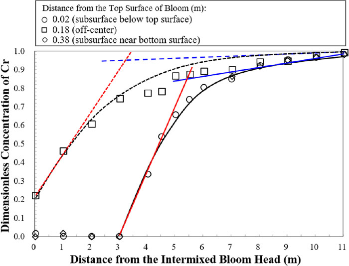
Comparison of the measured concentration of chromium on the the subsurface and the off-center positions from the first strand (WLMC = 8.26 ton, VLMC = 0.1 m/min). (Online version in color.)
Cho and Kim5) proposed a mixing prediction model consisting of three parameters to predict the concentration of a mixed portion. Two scale factors of the three parameters were applied to reflect the influence of the flow pattern affected by the morphology of the system such as the tundish and the mold. The concentrations of mixed molten steel flowing out from each system are obtained using scale factors, respectively. The scale factors are the parameters that affect the weighting factors to the concentration of molten steel flowing into the system and the average concentration of residual molten steel in the system. The scale factors can be tuned by reflecting the measured concentration of the mixed portion, suggesting that it may be the simplest, most efficient, and most practical among existing mixing prediction models for the different-grade continuous casting.
Their model has not distinguished the concentrations of the surface and the center of the mixed portion because their experimental data indicate that the concentration difference between the surface and the center of the mixed portion is not significant. However, as detailed in Section 2, the concentration distribution of the mixed portion exhibits different trends at the off-center and the subsurface of the solidified steel. If not only the concentration of the mixed portion of the surface but also that of the center can be accurately predicted through their model, the concept of applying scale factors can be extended to predict the inner concentration of the mixed portion. In order to predict the distinguished concentration of the mixed portion at the off-center and the subsurface of the solidified steel, three additional parameters should be introduced in their model.5) Hence, six parameters are required to predict the concentration of the solidified steel at the off-center and the subsurface based on the measured concentrations as shown in Fig. 6.
Figure 7 shows the results of applying the mixing prediction model by Cho and Kim5) to a 400×500 mm2 bloom. The zero point on the x-axis represents the position of the mold meniscus when new molten steel is introduced into the tundish. The blue solid lines shown in Figs. 7(a)–7(c) are the concentrations of the mixed portion when fTD = 1.0, fMD = 1.0, and L = 0.7, which are the optimal parameter values derived from their study.5) Figure 7(a) shows changes in the concentration of the mixed portion according to fTD. The slope is defined by the ratio of the concentration on the y-axis to the distance on the x-axis, when fTD > 1.0, the initial concentration of the mixed portion has a negative value with an initial negative slope. After passing through the inflection point of each line when fTD > 1.0, the lines exhibit a positive slope, whereby the concentration of the mixed portion gradually increases and changes from a negative to a positive value. However, when two different grades of molten steel are mixed in a state with concentrations of 0 for old molten steel and 1 for new molten steel, respectively, the concentration of the mixed portion if there is no phase change must be between 0 and 1. Thus, a negative concentration of the mixed portion cannot occur since the mixing prediction model does not take into account phase changes. If the fTD value used in Cho and Kim’s mixing model5) is greater than 1, the concentration of the mixed portion initially follows a negative value, and the negative value affects the concentration of the mixed portion in the calculation in the next step. The negative value can cause errors in the prediction results. To resolve this problem, the negative concentration of the mixed portion should be clipped to zero.

Predicted concentration of the mixed portion using the mixing model of Cho and Kim5) as a function of various parameters: (a) as a function of fTD ( 1.0;
1.0;  1.5;
1.5;  2.0;
2.0;  4.0;
4.0;  8.0) at fMD = 1.0 and L = 0.7; (b) as a function of fMD (1.0; 0.5; 1.5; 2.0; 4.0;
  8.0) at fTD = 1.0 and L = 0.7; and (c) as a function of L (0.7; 0.01; 1.0; 2.0; 4.0; 8.0) at fTD = 1.0 and fMD = 1.0. (Online version in color.)
Distances from the mold meniscus which start to have the positive concentration of the mixed portion (hereinafter, referred to as the starting point) are different at the center and the surface of the mixed portion. Mixed molten steel injected into the mold from the tundish starts to be solidified by the cold walls of the mold. The concentration of the initial solidifying shell of the strand near the mold meniscus and the mold walls follows the changing history of the concentration of mixed molten steel flowing out from the tundish. Thus, the starting point at the surface is always a positive value because of the time delay until mixed molten steel in the tundish arrives in the mold after new molten steel enters the tundish. Whereas, mixed molten steel penetrated deep to the lower strand flows towards the center of the strand, and the concentration of the center of the lower strand is affected by the movement and the diffusion of mixed molten steel in the mold. The starting point at the center of the mixed portion implies the depth of mixed molten steel penetrated to the lower strand. Thus, the starting point at the center of the mixed portion is always smaller than the starting point at the surface of the mixed portion.
When new molten steel is poured into the tundish, the smaller the amount of residual molten steel in the tundish, the shorter the path of mixed molten steel moving from the tundish to the mold. The starting point at the surface of the mixed portion is a small positive value because of the short path of mixed molten steel flowing out from the tundish. Whereas, the starting point at the center of the mixed portion is negative value because of the movement of mixed molten steel penetrated deep to the lower strand after being delivered to the mold.
However, if the amount of residual molten steel in the tundish is larger, the starting point at the surface of the mixed portion becomes a larger positive value owing to the longer path of mixed molten steel moving from the tundish to the mold. The starting point at the center of the mixed portion may be a small positive value owing to the restricted penetration depth of mixed molten steel in the mold and the long path of mixed molten steel in the tundish. Therefore, the starting point at the center of the mixed portion may be a positive or a negative value according to the amount of residual molten steel in the tundish when new molten steel is injected into the tundish. The mixed portion that does not satisfy the allowable range of concentration of old or new molten steel in the entire cross-section of the mixed portion must be scrapped or downgraded. Thus, it is important to find the starting points according to the location in the cross-section of the mixed portion.
In Fig. 7(a), when fTD = 1 and fTD = 4, the distances at which the concentrations are changed from negative to positive values (starting points) are −0.7 m and at 0 m, respectively. When fTD > 4.0, the starting point is a positive value. With a large fTD value, the starting point gradually increases. The difference between the starting points of fTD = 2.0 and fTD = 4.0 is similar to that of fTD = 1.0 and fTD = 2.0, but the difference between the starting points of fTD = 4.0 and fTD = 8.0 is smaller than that of fTD = 2.0 and fTD = 4.0. Even if the fTD value gradually increases by two times, the difference between the two starting points starts to decrease. This implies that the starting point cannot be significantly increased even if fTD is large. The difference of the starting points between the off-center and the subsurface is more than 3 m as shown in Fig. 6, but the difference between the starting points of fTD = 1.0 and fTD = 8.0 is approximately 1 m. Thus, the mixing prediction model cannot predict the difference of the measured starting points, even if small fTD and relatively large fTD values are applied for calculation of the concentrations of the mixed portion at the off-center and the subsurface, respectively.
At the same distance in the x-axis, the measured concentration of the mixed portion at the subsurface is not always greater than that at the off-center as shown in Fig. 6. In Fig. 7(a), the concentration of the mixed portion at fTD = 1.0 is larger than that at fTD = 8.0 when the distance is smaller than 1.5 m, but the concentration of the mixed portion at fTD = 1.0 is smaller than that at fTD = 8.0 when the distance is larger than 1.5 m. The predicted concentration of the mixed portion at a relatively large fTD value is smaller than that at a small fTD value in a specific range of the distance, but the opposite result is shown as the distance increases beyond the specific range of the distance as shown in Fig. 7(a). Thus, the mixing prediction model cannot predict the phenomenon that the concentration of the mixed portion at the off-center is always larger than that at the subsurface, even if small fTD and relatively large fTD values are applied for calculation of the concentration of the mixed portion at the off-center and the subsurface. Therefore, adjusting fTD value in the mixing prediction model cannot reflect the measured results shown in Fig. 6.
The positive slope gradually decreases as the distance increases as shown in Fig. 7(a). The slope at the starting point of a relatively large fTD value is always greater than the slope at the starting point of a small fTD value. If small fTD and relatively large fTD values are applied to the calculation of the concentration of the mixed portion at the off-center and the subsurface, respectively, then the slope at the starting point of the off-center is smaller than the slope at the starting point of the subsurface. Therefore, adjusting fTD value cannot reflect the slope at the starting point of the off-center greater than the slope at the starting point of the subsurface as shown in Fig. 6.
Figure 7(b) shows changes in the concentration of the mixed portion according to fMD. The starting point at fMD = 1.5 is greater than that at fMD = 1.0, but that at fMD = 8.0 is smaller than that at fMD = 4.0. With a large fMD value, the starting point generally increases, but the starting point starts to decrease when fMD is larger than a specific value. Regardless of fMD value, the starting point is always a negative value. When fMD > 1.0, the concentration of the mixed portion starts to oscillate as the distance increases. The larger fMD value, the faster and the stronger oscillation of the concentration of the mixed portion. These fMD characteristics exhibit a different tendency from those of fTD. The starting point cannot be significantly increased even if fMD is large. At the same distance, the concentration of the mixed portion at a relatively large fMD value is initially smaller than that at a small fMD value, but the opposite phenomenon occurs as the distance increases. These fMD characteristics exhibit a similar tendency to those of fTD.
Figure 7(c) shows the concentration of the mixed portion according to L, which is related to the amount of the molten steel that affects a mixing in the mold or the strand. The L value of 0.01 indicates that the length from the mold meniscus affecting the mixing of molten steel in the strand is 10 mm. Therefore, the L value must be greater than zero. Unlike the characteristics of fTD and fMD, as L is increased, the starting point is decreased, and the initial positive slope becomes small. The starting point is dominantly determined by the L value. When fTD = 1.0 and fMD = 1.0, the starting point is equal to −L value as shown in Fig. 7(c). At the same distance, the concentration of the mixed portion at a relatively large L value is initially greater than that at a small L value, but the opposite phenomenon occurs as the distance increases like the characteristics of fTD and fMD.
Therefore, based on the results presented and discussed in this section, the characteristics and limitations of the parameters used in the mixing model of Cho and Kim5) limit its ability to predict the mixed portion with a large concentration difference between the off-center and the subsurface of solidified steel shown in Fig. 6.
Figure 8 shows that flow patterns of molten steel in the tundish and the strand are changed according to the geometry-related factor of each system and the operating conditions of the continuous caster in the present study. The flow field in a system with inflow and outflow of the fluid can be generally divided into stagnant, mixed, and plug flow regions in the steady and unsteady states.18,19,20,21,22,23,24,25,26,27,28,29) The volume ratio of each region to the total volume of the system is decided by geometry-related factors and operating conditions of the system in the steady state. The concentration of the total volume consisting of stagnant, mixed, and plug flow volumes in the system can be assumed to have an average concentration. If the total volume of the system is changed owing to the difference of the amount of inflow and outflow over time, each volume ratio is changed in the transient state. If a concentration of the fluid flowing into the system is different from the concentration of the remained fluid in the system, the average concentration of the fluid in the total volume is changed owing to the concentrations of the fluid flowing into the system and the fluid flowing out from the system, and the concentration of the remained fluid in the system. Thus, the average concentration of the fluid in the total volume is determined by the amount of each fluid and the concentration of each fluid.

Schematic diagram of fluid flow in the tundish and the strand. (Online version in color.)
If the flow of molten steel is symmetric in two outlets of the tundish, the concentration of mixed molten steel in outflow at each outlet will be the same. However, if the asymmetric flow is caused by two or more asymmetric outlets arranged in a system, the concentration of mixed molten steel at each outlet may not be the same because the degree of influence by the interaction between each volume is locally different. Hence, the concentration of mixed molten steel at each outlet of the system having asymmetric flow may be different. Therefore, the local average concentration of mixed molten steel in the system must be introduced to apply individually to each outlet as follows:
| (2) |
The volumetric flow rate flowing into the tundish is a function of the weight change in the tundish and the volumetric flow rate flowing out of the tundish, as follows:
| (3) |
| (4) |
The flow rate flowing out from each mold to the strand can be obtained through the following equation:
| (5) |
The concentration of molten steel flowing out from the tundish is determined as a function of the concentration of new molten steel flowing into the tundish and the average concentration of residual molten steel in the tundish as obtained by
| (6) |
If CTin = 1 and
Hot molten steel guided by the SEN and injected into the mold has various flow patterns depending on the shape of the SEN outlet, and begins to be solidified from the outer surface of the strand by the cold mold wall. Thus, the mixing in the mold and the strand is more complicated than that in the tundish. The flow pattern in the mold varies depending on the SEN’s outer diameter, inner diameter, immersion depth and direction, and the angle and the number of discharge holes of the SEN. In the present study, the SEN with four discharge holes of an upward angle was used.
A part of the molten steel discharged from the outlet of the SEN exhibits a wide spread in the meniscus direction by the inert gas injected into the SEN. As the solidification proceeds from the meniscus, the concentration of the solidified shell at the strand surface is determined by the concentration of moving flow in the meniscus direction. Subsequently, most of molten steel hits the solidifying shell near the mold wall, and is divided into downward flow by gravity and upward flow by inertia. The downward flow moves toward the center of the strand as it descends deeper. In addition, in the moving flow toward the center of the strand, some of molten steel moves in the upward direction. In other words, the inner concentration of the solidified steel is determined by the downward and upward flow of some mixed molten steel as descending mixed molten steel moves to the center of the strand. As a result, after the solidification of the strand is complete, the concentration of the mixed portion is determined by the flow pattern inside the mold and the strand, and depends on the location of the cross-section in the intermixed bloom.
Since the amount of inflow into the strand and the amount of outflow from the strand are approximately equal in the mold, it can be assumed that only a limited region of the strand affects the concentration of the solidified steel due to the flow pattern inside the strand. Thus, assuming a simple hexahedron flow region within the strand with a rectangular cross-section, the limited flow region is a function of the distance from the mold meniscus. Figure 10 shows the schematic diagram of flow regions within the strand that affect the concentration of the mixed portion at the subsurface and the off-center. The flow regions within the strands that affect the concentration of the mixed portion at the subsurface and the off-center in the intermixed bloom are expressed by Eqs. (7) and (8), respectively:
| (7) |
| (8) |
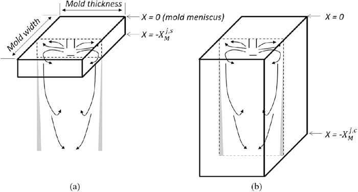
Schematic diagram of the flow regions within the strand that affect the concentration of the mixed portion: (a) at the subsurface and (b) at the off-center.
Therefore, the average concentration of molten steel in the mold is expressed by Eqs. (9) and (10):
| (9) |
| (10) |
| (11) |
The concentrations of molten steel in outflow from each flow region of the j-th strand are expressed as Eqs. (12) and (13), respectively:
| (12) |
| (13) |
Finally, the position with the calculated concentration of the molten steel in the outflow from each flow region should be adjusted to the position with the measured concentration of the finally solidified steel in the intermixed bloom, as follows:
| (14) |
| (15) |
Calculation procedure of the proposed mixing model.
The parameters of the mixing prediction model proposed in the present study are determined based on the measured concentration results. The parameters that affect the calculation of concentration of the mixed portion at the subsurface must be determined before determining the values of parameters at the off-center.
First of all,
Next,
If
In order to select or adjust the values of the appropriate parameters, it is necessary to examine the characteristics of each parameter in detail as in section 5.2.
5.2. Characterization of the Proposed Mixing ModelFigures 11, 12, 13 show the prediction results of the concentration of the mixed portion in the intermixed bloom of the first strand (j = 1). A value of zero on the x-axis indicates the position of the mold meniscus when the supply of new molten steel into the tundish begins, and a positive value on the x-axis indicates the position of the as-cast steel already produced at that time as a lower position than the mold meniscus. Therefore, a negative value means the position where the molten steel that remained within the tundish when new molten steel is supplied to the tundish flows out from the tundish, and solidifies. The blue solid line displays the predicted concentration of the mixed portion when
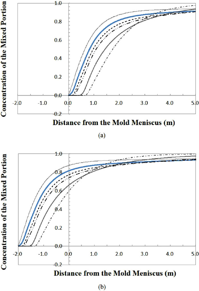
Predicted concentration of the mixed portion as a function of 1.0; 0.5; 1.5; 2.0; 4.0; 8.0. (Online version in color.)

Predicted concentration of the mixed portion as a function of 1.0; 0.5; 1.5; 2.0; 4.0; 8.0. (Online version in color.)

Predicted concentration of the mixed portion as a function of 0.7; 0.01; 1.0; 2.0; 4.0; 8.0. (Online version in color.)
Figure 11(a) shows the change in the predicted concentration of the mixed portion according to
The distance is positive for all
The difference of the starting points between the center and the surface is significantly different as shown in Fig. 6, but the predicted result by adjusting
Figure 12(a) shows the change in the predicted concentration of the mixed portion according to
The predicted result by adjusting
Figure 13(a) shows the change in the predicted concentration of the mixed portion according to
Therefore, the newly proposed mixing model in the present study exhibits flexibility in predicting the concentration of the mixed portion. Figure 14 shows the predicted concentration of the mixed portion in the off-center and the subsurface of the intermixed bloom when appropriate values of the parameters are applied to the present model. Good agreement between the predicted and the measured results is observed by adjusting the additional parameters introduced in the present study.

Prediction of the subsurface and the off-center concentrations in the intermixed bloom of the first strand.
Various flow patterns in the tundish and the mold may occur depending on different factors, such as the internal shape and operating conditions of the continuous casting machine. The measured concentrations of the mixed portion in the intermixed bloom are attributed to various flow patterns in different-grade continuous casting. Therefore, the mixing prediction model using scale factors developed based on the measured concentration reflects the influence of various flow patterns by adjusting the scale factors and thus has high accuracy.
The mixing prediction model proposed in the present study uses scale factors
Figure 15 shows the prediction and the measurement results of the subsurface concentrations of the mixed bloom from the first to the fourth strand. When the strand numbers are 2, 3 and 4 (j=2,3,4), only the concentration of the mixed portion at the subsurface was measured. Since the change in the casting speed of each strand was the same, the calculated results of each strand are also the same. Therefore, only the calculated curve of the first strand is shown in Fig. 15. Even considering the limited measurement data of the subsurface concentration, the concentration of the mixed portion for the same position of each strand in the length direction is quite similar to each other, and all the parameters used in the mixing prediction model for each strand can be applied identically. The values of parameters to be applied differently for each strand can be set with an equal value through this result, but since there are many events such as break-out by the tearing of the solidifying shell or stoppage of a specific strand by clogging of the submerged entry nozzle, it is necessary to predict the concentration of the mixed portion in each strand.
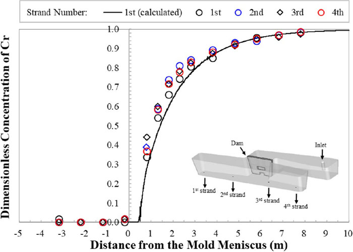
Prediction and measurement results of the subsurface concentration in the intermixed bloom from the first to the fourth strand. (Online version in color.)
Prediction of the inner concentration of the mixed portion can be required to properly treat the mixed portion that does not satisfy the criteria for the concentration of the steel grades. In other words, it may be more desirable to predict the maximum and the minimum concentrations of the mixed portion throughout the cross-section than to predict only the concentrations of the mixed portion at the off-center and the subsurface. The superscripts s and c of Eqs. (7) and (8) can be changed to the superscripts min and max depending on the user’s purpose. Figure 16 shows the results of the predicted maximum and minimum concentrations of the mixed portion at the entire cross-section in the intermixed bloom from the first strand (j = 1) when
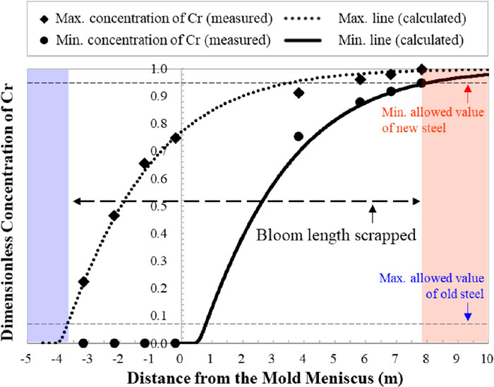
Prediction of the minimum and the maximum concentrations of the mixed portion in the intermixed bloom of the first strand. (Online version in color.)
To predict the concentration of the mixed portion using various models such as physical models, and numerical analyses is often expensive in terms of computational cost. Furthermore, these methods should be simplified through assumptions, and various parameters may be introduced to verify the obtained results. If the geometry-related factors of the system that affect the flow pattern vary, additional efforts for developing and validating the model will be required. The most reliable approach to validate the prediction results of the models is to directly measure the concentration of the mixed portion. The mixing prediction model using scale factors can reflects the influence of flow patterns based on the measured concentration of the mixed portion effectively. The mixing prediction model proposed in the present study is practical and accurate because it can directly reflect the measurement results.
The mixing prediction model of Cho and Kim5) calculates the concentration of the mixed portion using scale factors related to the geometry of the system based on a simple flow phenomenon of the molten steel entering and leaving the system. Compared to other previous mixing prediction models, their model5) has an advantage of using the lowest number of parameters. At the same time, their model5) has a disadvantage in that the reliability of the predicted concentration of the mixed portion is low when the concentration difference between the surface and the center is large in the intermixed slab or the intermixed bloom with a large cross-section.
In the present study, the concentrations of the mixed portion were measured along the length and the thickness directions of the intermixed bloom, and the changing trend was analyzed in detail. In addition, the characteristics and limitations of Cho and Kim’s mixing prediction model5) using scale factors were investigated. Through the investigation, a new flexible, fast, and accurate mixing prediction model has been developed to predict the concentration of the mixed portion at the surface and the center of the intermixed bloom by utilizing the advantages of the mixing prediction model using scale factors.
The new mixing prediction model has been validated by measuring the concentration of the mixed portion of many intermixed blooms.
The main conclusion of the present study can be summarized as follows:
(1) Concentrations of the mixed portion generated by different-grade continuous casting were measured in the intermixed bloom along the thickness direction at each longitudinal position. The measured concentration of the mixed portion significantly varied based on the cross-sectional location. In particular, at the same distance, the maximum and the minimum concentrations of the mixed portion in the cross-section do not necessarily occur only at the surface and the center of the intermixed bloom. Therefore, a mixing prediction model must be developed to predict the maximum and the minimum concentrations of the mixed portion at the cross-section along the length direction of the intermixed bloom.
(2) Based on the measured concentration of the mixed portion, a practical, flexible, fast, and accurate mixing prediction model using scale factors related to the geometry of the system has been developed. The newly proposed mixing prediction model can be used to predict the concentrations of the mixed portion in a continuous caster with multiple strands exhibiting asymmetric flow. Furthermore, the proposed mixing model shows good compatibility for predicting the experimental results by adjusting the additional parameters introduced in this study.
(3) The present mixing prediction model has been found to predict accurately the concentration profiles of the mixed portion along the surface and the off-center of the intermixed bloom. Moreover, it can be used to predict the maximum and the minimum concentrations of the mixed portion in the cross-section of the intermixed bloom along the length direction.