Multiphase Modeling of Steel-slag Mass Transfer through Distorted Interface in Bottom-stirred Ladle

Abstract

A three-dimensional computational fluid-dynamics (CFD) model containing three phases: water, oil, and air was developed to study the mass transfer process at the slag-steel interface in the ladle. The transient mass transfer between slag and metal phases occurred only at the interface and the transient irregular distorted interface was considered. A more realistic concentration distribution and transient variation process of mass transfer in the bottom-blown ladle was obtained.

1. Introduction

Ladle furnace (LF) is an important process to ensure the steel quality and improve the production efficiency. Most metallurgical reactions, such as desulfurization, involve three steps: diffusion of reactant species to the slag/metal interface, interfacial reaction, and diffusion of reaction products into the slag phase.¹⁾ Blowing gas to stir the ladle promotes the temperature and composition uniformity of the molten steel, accelerates metallurgical reactions, advances alloy melting, and removes non-metallic inclusions in the steel, which effectively promotes the quality of steel products, improves the ladle refining efficiency, and reduces the production costs.^2,3,4) Due to the high temperature condition in the actual production process, it is commonly assumed that the rate limiting step of most metallurgical reactions is the mass transfer between the slag-steel phases rather than the interfacial chemical reaction. The inert gas blown through the bottom of the vessel causes a rising gas/liquid plume, which induces recirculation movement in the molten bath and fluctuations at the slag-steel interface.⁵⁾ The actual mass transfer process occurs at the fluctuating steel-slag interface.

In previous studies, certain assumptions (usually associated with the cross-sectional area of the vessel) were made about interfacial area by some scholars in order to investigate the factors influencing mass transfer coefficient. Additionally, some studies utilized volume mass transfer coefficient (the product of mass transfer coefficient and interface area) as their analysis target.^{1,6,7,8,9,10,11,12,13,14,15)} Among them, the mass transfer coefficient (or volume mass transfer coefficient) was typically expressed as a function of variables such as stirring power and blowing flow rate.^16,17,18,19) Although the volumetric mass transfer coefficient could be used to assess the factors affecting the mass transfer rate between two phases, it was challenging to precisely determine the quantitative impact of various factors on either the mass transfer coefficient or the interface area.

Some numerical models have been developed in the last decades.^{4,20,21,22,23,24,25,26,27,28)} Jonsson et al.^20,21) proposed a numerical model coupling CFD and thermodynamics to study the desulfurization process in gas-stirred ladles. The model was a two-dimensional model considering steel, slag, and argon phases, where the movement of elements between the slag and metal phases were represented using source/sink terms. The source terms of different elements were linked by assuming a finite number of chemical reactions. It was assumed in the model that for any appropriate time step, the thermodynamic equilibrium was reached before the end of the time step due to the adequate mixing of slag and metal at the interface. Lou et al.^4,22) developed a CFD simultaneous reaction (CFD-SRM) coupling model to describe the desulfurization behavior in a gas-stirred ladle, the mass transfer between the slag and metal phases were also represented by source/sink terms. The interface area of slag-metal in their CFD model was the sectional area of the ladle minus the slag eye area, of which the slag eye area was calculated using empirical formulas. The mass transfer coefficient has usually been calculated based on Lamont’s model.²⁹⁾ Only the liquid steel phase was included in Lou’s research and the interface area remained unchanged in the calculation process. Later on, Cao et al.^23,24) proposed a fully transient 3D CFD model including gas, slag, and steel, in which the instantaneous slag-steel interface area was used to calculate mass transfer process. However, in most numerical models, the overall mass transfer of the liquid steel phase was calculated and the average mass source term was applied to the entire bulk steel instead of being specifically targeted towards the slag-steel interface.

The main objective of the present study was to establish a three-dimensional CFD numerical model containing three phases, where the mass transfer of two phases occurred only at the interface and the transient irregular distorted interface was considered. Due to the high temperature environment, it was difficult to obtain the data of the actual ladle. Therefore, the physical model of the gas-stirred ladle was developed using water, oil, and air, then the numerical model was established on this basis.

2. Physical Model

The water model with a geometric scale of 1:10 corresponding to 210 tons of industrial ladle was employed to carry out the experimental work, as shown in Table 1. The schematic diagram of the experiment is shown in Fig. 1(a). The blowing porous plug is located in the center of the bottom of the ladle. The modified Froude number was considered as the similarity criterion for correlating the gas flow rate between the scale model and the full-scale system, the details was descripted in the previous literature.³⁰⁾

Table 1. Dimensions of prototype and water model.

Dimensions/variables	Prototype (m)	Water model (m)
Diameter of bottom	3.513	0.351
Diameter of top	3.900	0.390
Total height	5.000	0.500
Height of liquid steel	2.810	0.281
Thickness of slag	0.08	0.008
Porous plug diameter	0.13	0.013

Fig. 1. Schematic of the water model. (Online version in color.)

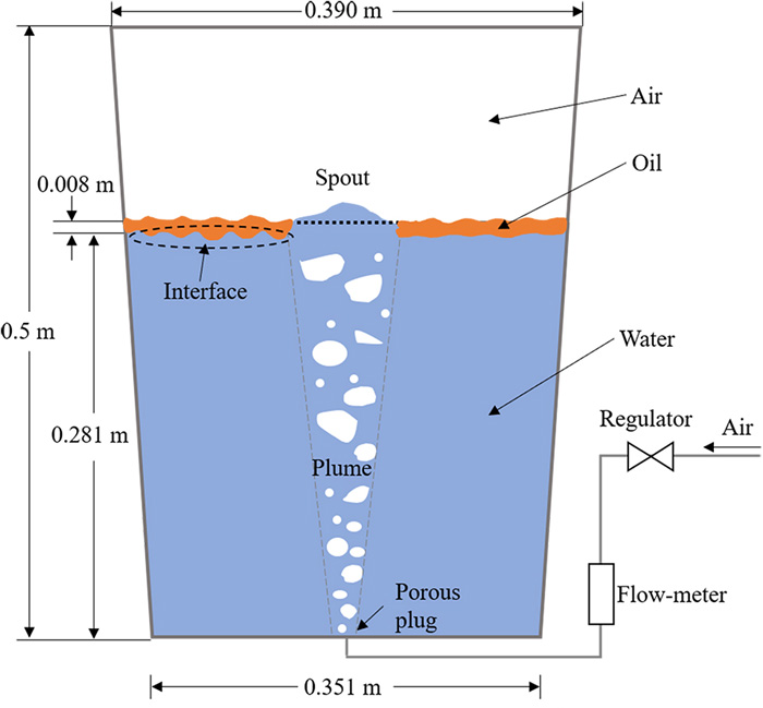
Based on the authors’ previous work,³¹⁾ deionized water, petroleum ether, and air were chosen as the liquid steel phase, slag phase, and blown-in argon phase, respectively. Thymol was used as a mass transfer tracer to simulate the transfer from the aqueous phase to the oil phase. Typically, 0.281 m high deionized water was added to the ladle model, and then thymol reagent was added to configure a mixed aqueous solution with an initial thymol content of 100 ppm (ppm is mg/kg in present study). Then 0.92 L of petroleum ether, which corresponds to an 8 mm thick oil layer, was added, then started to inject gas at the bottom of ladle. After starting gas stirring, the sample was taken out from the water on the upper part of the ladle using a long dropper at regular intervals. The samples were analyzed with a UV spectrophotometer to determine the concentration of thymol in the water.

3. Numerical Model

The experimental water model was chosen as the object of simulation, the dimensions of which are shown in Fig. 1 and Table 1. The governing equations for continuity, momentum, and turbulence were solved using the CFD commercial code ANSYS FLUENT 2020R2. The mathematical model is based on the Euler-Lagrangian (E-L) reference frame, using VOF to track the dynamic position of the interface between different phases; DPM model was used to describe the bubble movement and interphase forces, including lift, drag, virtual mass forces and pressure gradient force. Species model was used to calculate thymol transfer between water phase and oil phase. The control equations of continuity, momentum, turbulence and DPM models are shown in the reference.³²⁾ The control equations for mass transmission are as follows:³³⁾

For the i^th species, the convection-diffusion equation takes the following general form:

  

$$\frac{\partial }{\partial \text{t}}\left(\rho {\text{Y}}_{\text{i}}\right)\text{+}\nabla \cdot \left(\rho \overrightarrow{\mathrm{v}}{\mathrm{Y}}_{\mathrm{i}}\right)=\nabla \cdot \left(\left(\rho {\text{D}}_{\text{i,m}}+\frac{{\mu }_{\text{t}}}{{\text{Sc}}_{\text{t}}}\right)\nabla {\text{Y}}_{\text{i}}\right)+{\text{S}}_{\text{i}}$$(1)

where Y_i is the local mass fraction of each species; D_i,m is the mass diffusion coefficient for species in the mixture; Sc_t is the turbulent Schmidt number and the default value is 0.7. S_i is the mass transfer source term of species i, here it is a user-defined sources which will be described in the next section.

3.1. Mass Transfer through Water-oil Interface

As shown in Fig. 2(a), the mass transfer of Thymol between water and oil only occurred at the distorted interface between the top water and oil layers, where the mass transfer source term S_i in Eq. (1) existed only at the interface. As mentioned earlier, most numerical models didn’t limit the two-phase mass transfer to the interface or considered irregular interfaces. The current work attempts to overcome these shortcomings and establish a transient mass transfer model between water and oil phases. As shown in Fig. 2(b), at any time, the water-oil interface was composed of a certain number of local interfaces, each with different concentrations and local flow states, leading to different thymol transfer quantities. In the numerical model, the mass transfer process at the water-oil interface was transformed into a mass transfer problem of the interface grid, and the difference in local interfaces was transformed into the difference in mass source terms of each grid at the interface, as shown in Fig. 2(c).

Fig. 2. Schematic diagram of mass transfer at (a) deformed oil-water interface (b) local oil-water interface (c) cell of interface. (Online version in color.)

The mass source term S_i at any time on the interface grid can be expressed as:

  

$${\text{S}}_{\text{i}}={\text{J}}^{\text{cell}}\frac{{\text{A}}^{\text{cell}}}{{\text{V}}_{\text{w}}^{\text{cell}}}$$(2)

  

$${\text{J}}^{\text{cell}}={\text{k}}_{\text{eff}}^{\text{cell}}\left({\text{C}}_{\text{w}}^{\text{cell}}-\frac{{\text{C}}_{\text{o}}^{\text{cell}}}{\text{h}}\right)={\text{k}}_{\text{eff}}^{\text{cell}}\left({\rho }_{\text{w}}{\text{[wt\%]}}_{\text{w}}^{\text{cell}}-\frac{{\rho }_{\text{o}}{\text{(wt\%)}}_{\text{o}}^{\text{cell}}}{\text{h}}\right)$$(3)

  

$${\text{k}}_{\text{eff}}^{\text{cell}}=\frac{\text{1}}{1/{\text{k}}_{\text{w}}^{\text{cell}}+1/\left({\text{hk}}_o^{\text{cell}}\right)}$$(4)

where the superscript “cell” represents a cell, and the subscripts “w” and “o” represent water phase and oil phase, respectively. J denotes mass transfer flux density (kg·m⁻²·s⁻¹), A represents interface area (m²), V is volume (m³); k and k_eff are mass transfer coefficients and effective mass transfer coefficients (m·s⁻¹), C denotes mass concentration (kg·m⁻³); [wt%] and (wt%) represent the mass fraction in water and oil, respectively; h is the partition ratio of mass concentration in the oil phase to that in the water phase at the final equilibrium state, which has been experimentally measured as 23 (the corresponding partition ratio of mass fractions was 35) in this study.

In Eqs. (2), (3), (4), the volume and mass fraction in the oil and water phases within the interfacial cells can be read by user define function (UDF) in Fluent. The mass transfer coefficient and interfacial area calculation methods are described as follows.

The mass transfer coefficient is calculated using the eddy cell model proposed by Lamont and Scott,²⁹⁾ which can be expressed by the following equation:

  

$${\text{k}}_{\text{l}}=\text{0}\text{.4}{\left(\frac{{\nu }_{\text{l}}}{{\text{D}}_{\text{l}}}\right)}^{-\text{1/2}}{\left(\frac{{\epsilon }_{\text{l}}}{{\nu }_{\text{l}}}\right)}^{\text{1/4}}$$(5)

where, l represents the liquid phase (water or oil), ν is the dynamic viscosity (m²·s⁻¹), D is the diffusion coefficient (m²·s⁻¹), and ε is the turbulent dissipation rate (m³·s⁻²).

The geometric reconstruction method is a commonly used interface reconstruction scheme in the VOF method, which represented the interface between fluids with a piece wise linear approach (Piecewise Linear Interface Calculation, PLIC). Song et al.³⁴⁾ proposed a method for calculating the interface area between the two phases in a 3D straight hexahedron cell based on the PLIC method. They flipped and symmetrized the coordinate system based on the normal vector of the reconstructed phase interface and the dimension of the mesh cell, then simplified the interface types into five categories, as shown in Fig. 3. The relevant numerical methods were used to determine the plane equation where the reconstructed phase interface was located, and thus obtained the area of the phase interface (pink shadow surface in Fig. 3 within the computable cell. In this paper, the method proposed by Song et al. was used to calculate the area of the interface within each interface cell, using the planar area in Fig. 2(c) as a substitute for the actual curved surface area.

Fig. 3. Five generic types of interface configuration (adapted from ref.³⁴⁾). (Online version in color.)

In summary, the mass transfer calculation process of thymol between water and oil in each calculation step is shown in Fig. 4. Here, the UDF was used to achieve these goals. Some data such as the geometric size, volume, volume fraction, thymol concentration, turbulent dissipation rate of the cell could be accessed directly from the model, while the gradient vector, the two-phase interface area and the mass transfer coefficient in the cell were calculated based on the accessed data. In addition, it should be noted that the method of calculating the interface area in the cell proposed by Song et al. was specifically applied to regular hexahedron cells. Therefore, the structural meshes was used to divide the calculation domain in this study, and the proportion of cells with a Jacobian ratio greater than 0.9 was 96.43%.

Fig. 4. The solution schematic of mass transfer between water and oil at each calculation step.

3.2. Initial and Boundary Conditions

The model includes three phases: water, oil, and air, with specific physical properties shown in Table 2. The diffusion coefficients of thymol in the water and oil phases were calculated using the formula proposed by Wilke and Chang.³⁵⁾ The mesh and boundary of the numerical model are shown in Fig. 5, with higher mesh density in the oil phase region. The side and bottom walls were set as wall boundaries with no-slip and standard wall equations, while the top was set as a pressure-outlet. The initial velocities of water, oil, and air are zero. The initial concentration of thymol in water is 100 ppm, and it is 0 ppm in oil. The numerical simulation process involves first calculating the flow field for 60 seconds due to air agitation before adding petroleum ether and then solving the mass transfer equation simultaneously with the flow field to calculate the mass transfer between water and oil. This is because the actual water model experiment adds petroleum ether after stirring with air for a certain period of time.

Table 2. The physical parameters in the model.

Density of water	998.2 kg∙m−3
Density of petroleum ether	640 kg∙m−3
Density of air	1.225 kg∙m−3
Viscosity of water	0.001 Pa·s
Viscosity of petroleum ether	0.0003 Pa·s
Viscosity of air	1.784×10−5 Pa·s
Diffusion coefficient of thymol in water	2.46×10−10 m2·s−1
Diffusion coefficient of thymol in petroleum ether	3.16×10−9 m2·s−1
Interfacial tension between water and air	0.0728 N·m
Interfacial tension between water and petroleum ether	0.0478 N·m

Fig. 5. The Schematic diagram and mesh of boundary condition. (Online version in color.)

Air was injected through a porous plug with 76 evenly distributed small holes of 0.8 mm diameter, and the gas flow rate was 1.8 L/min. After injecting into the liquid, bubbles appeared in different sizes and shapes through collision, growth, and breakage. Although some models existed to describe the behavior of bubbles in water, there was no unified model for determining bubble size in such systems. In this study, the surface blowing method in the DPM model was used, with the initial velocity and average diameter of bubbles calculated using Eqs. (6) and (7).³⁶⁾

  

$${\text{u}}_{\text{b}}=\frac{\text{Q}}{{\text{A}}_{\text{eff}}}$$(6)

  

$${\text{d}}_{\text{b}}=\text{0}\text{.091}\left(\frac{{\sigma }_{\text{w-air}}}{{\rho }_{\text{w}}}\right){\text{u}}_{\text{b}}^{\text{0}\text{.44}}$$(7)

Where u_b and d_b are the initial velocity and diameter of the bubble, respectively; Q is the blowing flow rate; A_eff represents the effective blowing area, i.e., the sum of the areas of all the small holes in the porous plug; σ_w-air indicates the surface tension between water and air.

3.3. Solution Procedures

The structural mesh of ladle was created using ANSYS ICEM software and the transient pressure-based solver was selected. Pressure-velocity coupling solver was employed using the algorithm scheme PISO. The PRESTO! scheme was chosen for the spatial discretization of pressure. The convergence criteria considered in this study were below 1×10^–4 for the scaled residuals. As shown in Fig. 6, different numbers of mesh were used for mesh sensitivity analysis, with mesh counts of 260000, 440000 and 680000. From Fig. 6, the number of grids was independent of the result when the number of meshes large than 440000, so the mesh with number of 440000 was chose as the optimal one for the current numerical simulation studies.

Fig. 6. Mesh sensitivity analysis. (Online version in color.)

4. Results and Discussion

4.1. Comparison of Model and Measured Results

The comparison between simulated and measured concentrations of thymol in water is shown in Fig. 7. When the air flow rate was 1.8 L/min, the concentration of thymol in water decreased from 100 ppm to around 58 ppm and reached equilibrium at approximately 210 minutes. The numerical simulation results were found to be consistent with the physical experimental measurements. The changes in thymol concentration in the oil phase was shown in Fig. 8, where the concentration increased from 0 to around 2030 ppm as the thymol content in water decreased. The rate of change in thymol content in both the oil and water phases gradually slowed down with increasing time.

Fig. 7. Comparison between calculated result and measured result. (Online version in color.)

Fig. 8. The average content of thymol in oil phase.

4.2. The Distribution of Thymol and Mass Source Term

The slag eye and the distribution of different phases at 100 min are shown in Fig. 9. It can be clearly seen that the top oil phase was blown open to form a slag eye due to the effect of bottom blowing gas, while there was a certain degree of deformation in the water-oil interface. The distribution of thymol concentration in each phase at different times are shown in Fig. 10. According to Fig. 10, the initial thymol concentration in oil was 0 ppm, and the thymol in water gradually transferred to the oil phase with the stirring of gas. The shape of the water-oil interface changed over time, and the distribution of thymol concentration in the oil phase was consistent with the distorted shape of the oil phase.

Fig. 9. The (a) slag eye and (b) distribution of different phases at 100 min. (Online version in color.)

Fig. 10. The thymol distribution at different time: (a) 0 min (b) 100 min, and (c) 200 min. (Online version in color.)

The distribution of the mass source term in the model at different times was shown in Fig. 11, and the result of local magnification of the mass source term distribution was also displayed in the figure. From the figure, it can be seen that the mass source term only existed at the distorted water-oil interface, and its value was 0 at the slag eye because the transfer of thymol between the water phase and the oil phase occurred only at the interface between the two phases, and there was no contact between water and oil at the slag eye. The gas blowing from the bottom center led to the turbulent dissipation rate maximal at the center and minimal near the boundary. Therefore, the mass source term at the water-oil interface was highest near the slag eye and gradually decreased with increasing distance from it. The thymol concentrations in the oil phase and the water phase moved to equilibrium percentage, and the mass source term continuously decreased accordingly with time.

Fig. 11. The mass source distribution at different time: (a) 0 min (b) 100 min (c) 200 min. (Online version in color.)

5. Summary

In this study, a physical model of a gas-stirred ladle was established using water, oil, and air, and a new 3D-CFD multiphase flow model was developed to investigate the mass transfer process at the slag-steel interface in the ladle. The mass transfer between the water and oil phases in the model occurred only at the interface and considered the transient irregular distorted interface. The transient mass transfer source term of the water-oil interface cell was calculated by reading the size, volume fraction, concentration, turbulent dissipation rate, and other parameters of the model grid through UDF. The simulation results of the model were in good agreement with experimental results and can accurately predict the concentration distribution of substances in the two phases. The mass source term was 0 at the slag eye and only existed at the interface between the two phases. The mass source term decreased with decreasing the turbulent dissipation rate and interphase equilibrium concentration difference.

The current model considered the transient mass transfer at the interface between the two phases, allowing for a more realistic concentration distribution and transient variation process of mass transfer in the bottom-blown ladle. It was capable of analyzing the mass transfer process of different components between the two phases separately by including different components in the model. Additionally, the current model could also estimate the corresponding mass transfer coefficient and interface area. When the blowing flow rate and the position of the porous plug were varied, the individual effects of these variables on the mass transfer coefficient and interface area could be analyzed independently.

Acknowledgments

The authors are grateful for support from the Fundamental Research Funds (Grant No. 06500108) from the University of Science and Technology Beijing, China.

Supporting Information

Movie S1. A transient distribution of the thymol concentration was recorded over a 225-minute period in both the water and oil phases. The thymol in the upper water phase preferentially transferred to the oil phase, which was due to the mass transfer only occurring at the phase interface. Movie S2. A transient distribution of the mass source in the model was recorded over 225 minutes. The mass source occurred exclusively at the irregular and distorted interface between the water and oil phases, and it exhibited variations in both time and location. This material is available on the Journal website at https://doi.org/10.2355/isijinternational.ISIJINT-2023-310.

References

• 1)   N.  Joubert,  P.  Gardin,  S.  Popinet and  S.  Zaleski: Metallurgical Research & Technology, 119 (2022), 109. https://doi.org/10.1051/metal/2021088
• 2)   W.  Lou and  M.  Zhu: ISIJ Int., 54 (2014), 9. https://doi.org/10.2355/isijinternational.54.9
• 3)   H.  Tang,  X.  Guo,  G.  Wu and  Y.  Wang, ISIJ Int., 56 (2016), 2161. https://doi.org/10.2355/isijinternational.ISIJINT-2016-360
• 4)   W.  Lou and  M.  Zhu: ISIJ Int., 55 (2015), 961. https://doi.org/10.2355/isijinternational.55.961
• 5)   A.  Senguttuvan and  G. A.  Irons: ISIJ Int., 57 (2017), 1962. https://doi.org/10.2355/isijinternational.ISIJINT-2016-589
• 6)   T.  Lehner: Canadian Metallurgical Quarterly, 20 (1981), 163. https://doi.org/10.1179/cmq.1981.20.2.163
• 7)   M.  Hirasawa,  K.  Mori,  M.  Sano,  A.  Hatanaka,  Y.  Shimatani and  Y.  Okazaki: Transactions of the Iron and Steel Institute of Japan, 27 (1987), 277. https://doi.org/10.2355/isijinternational1966.27.277
• 8)   M.  Hirasawa,  K.  Mori,  M.  Sano,  Y.  Shimatani and  Y.  Okazaki: Transactions of the Iron and Steel Institute of Japan, 27 (1987), 283. https://doi.org/10.2355/isijinternational1966.27.283
• 9)   S.  Kim and  R.  Fruehan: Metallurgical and Materials Transactions. B, 18 (1987), 381. https://doi.org/10.1007/BF02656157
• 10)   K.  Umezawa,  H.  Matsunaga,  R.  Arima,  S.  Tonomura and  I.  Furugaki: Tetsu-to-Hagané, 69 (1983), 1810. https://doi.org/10.2355/tetsutohagane1955.69.15_1810
• 11)   J.  Deng and  F.  Oeters: Steel Research, 61 (1990), 438. https://doi.org/10.1002/srin.199000376
• 12)   K.  Ogawa and  T.  Onoue: ISIJ Int., 29 (1989), 148. https://doi.org/10.2355/isijinternational.29.148
• 13)   S.  Kitamura,  T.  Kitamura,  K.  Shibata,  Y.  Mizukami,  S.  Mukawa and  J.  Nakagawa: ISIJ Int., 31 (1991), 1322. https://doi.org/10.2355/isijinternational.31.1322
• 14)   H.  Xie and  F.  Oeters: Steel Research, 66 (1995), 501. https://doi.org/10.1002/srin.199501162
• 15)   F.  Jiang,  Y. X.  Song and  G. G.  Cheng: Revue de Metallurgie. Cahiers D’Informations Techniques, 108 (2011), 465. https://doi.org/10.1051/metal/2011081
• 16)   A.  Conejo: Processes, 8 (2020), 1. https://doi.org/10.3390/pr8070750
• 17)   Y.  Qu: Journal of University of Science and Technology Beijing, 10 (2003), 1.
• 18)   A.  Urióstegui-Hernández,  P.  Garnica-González,  J. Á.  Ramos-Banderas,  G.  Solorio-Díaz and  C. A.  Hernández-Bocanegra: ISIJ Int., 62 (2022), 1189. https://doi.org/10.2355/isijinternational.ISIJINT-2021-514
• 19)   C.  Mao,  X.  Guo,  N. J.  Walla,  A. K.  Silaen,  V.  Thapliyal and  C. Q.  Zhou: Ironmak. Steelmak., (2023), 1. https://doi.org/10.1080/03019233.2023.2195308
• 20)   L.  Jonsson,  D.  Sichen and  P.  Jönsson: ISIJ Int., 38 (1998), 260. https://doi.org/10.2355/isijinternational.38.260
• 21)   M.  Andersson,  M.  Hallberg,  L.  Jonsson and  P.  Jönsson: Ironmak. Steelmak., 29 (2002), 224. https://doi.org/10.1179/030192302225004106
• 22)   W.  Lou and  M.  Zhu: Metallurgical and Materials Transactions B, 45 (2014), 1706. https://doi.org/10.1007/s11663-014-0105-0
• 23)   Q.  Cao and  L.  Nastac: Metallurgical and Materials Transactions B, 49 (2018), 1388. https://doi.org/10.1007/s11663-018-1206-y
• 24)   Q.  Cao,  L.  Nastac,  A.  Pitts-baggett and  Q.  Yu: Metallurgical and Materials Transactions B, 49 (2018), 988. https://doi.org/10.1007/s11663-018-1234-7
• 25)   U.  Singh,  R.  Anapagaddi,  S.  Mangal,  K.  Padmanabhan and  A.  Singh: Metallurgical and Materials Transactions B, 47 (2016), 1804. https://doi.org/10.1007/s11663-016-0620-2
• 26)   Q.  Hoang,  M.  Ramírez-Argáez,  A.  Conejo,  B.  Blanpain and  A.  Dutta: JOM, 70 (2018), 2109. https://doi.org/10.1007/s11837-018-3056-0
• 27)   N.  Joubert,  P.  Gardin,  S.  Popinet and  S.  Zaleski: Metall. Res. Technol., 119 (2022), 109. https://doi.org/10.1051/metal/2021088
• 28)   Y.  Liu,  M.  Ersson,  H.  Liu,  P. G.  Jönsson and  Y.  Gan: Metallurgical and Materials Transactions B, 50 (2019), 555. https://doi.org/10.1007/s11663-018-1446-x
• 29)   J.  Lamont and  D.  Scott: AIChE Journal, 16 (1970), 513. https://doi.org/10.1002/aic.690160403
• 30)   A.  Conejo,  G.  Zhao and  L.  Zhang: Metallurgical and Materials Transactions B, 52 (2021), 2263. https://doi.org/10.1007/s11663-021-02170-1
• 31)   K.  Niu,  W.  Feng and  A.  Conejo: Metallurgical and Materials Transactions B, 53 (2022), 1344. https://doi.org/10.1007/s11663-022-02499-1
• 32)   K.  Niu,  W.  Feng,  A. N.  Conejo,  M. A.  Ramírez-Argáez and  H.  Yan: Metallurgical and Materials Transactions B, 54 (2023), 2066. https://doi.org/10.1007/s11663-023-02816-2
• 33)  ANSYS_Fluent, https://ansyshelp.ansys.com/, (2020), 571.
• 34)   Y.  Song,  Z.  Liu,  Y.  Tao,  X.  Peng and  Z.  Chen: Chinese Journal of Engineering, 38 (2016), 1091 (in Chinese). https://kns.cnki.net/kcms/detail/10.1297.tf.20160830.1031.001.html
• 35)   C.  Wilke and  P.  Chang: Aiche Journal, 1 (1955), 264. https://doi.org/10.1002/aic.690010222
• 36)   G.  Chen,  S.  He and  Y.  Li: Metallurgical and Materials Transactions B, 48 (2017), 2176. https://doi.org/10.1007/s11663-017-0992-y