Abstract
The mass transfer in the concentration boundary layer is often the rate-determining step for solid-liquid chemical reactions. Decreasing the concentration boundary layer thickness is essential to intensify the solid-liquid chemical reaction. Because convection contributes to decreasing the concentration boundary layer thickness, traditional methods excite a macro-scale flow in the bulk region. Since the concentration boundary layer exists in the velocity boundary layer near the solid-liquid interface, the traditional methods have limitation in enhancing the mass transfer. Based on this reason, the direct flow excitation near the solid-liquid interface by imposing an electromagnetic force was proposed. The aim of this research is to evaluate the effect of the time-varying electromagnetic force and its frequency on the mass transfer near the solid-liquid interface by evaluating the effective diffusion coefficient. The effective diffusion coefficient was evaluated under the imposition of a static electromagnetic force or a time-varying electromagnetic force with a frequency of 2 Hz or 6 Hz. The results found that by imposing the time-varying electromagnetic force, the mass transfer was enhanced compared to that under the imposition of the static electromagnetic force. The mass transfer was further enhanced by decreasing the time-varying electromagnetic force frequency.
1. Introduction
For solid-liquid chemical reactions, the mass transfer in a concentration boundary layer formed near the solid-liquid interface is often the rate-determining step, such as a refining process in the metallurgical industry and an electroplating process in the surface treatment industry.1,2,3,4) The mass transfer in it depends on diffusion and convection.1,4,5) The intensity of diffusion positively relates to the diffusion coefficient and the concentration gradient as described by Fick’s first law.6) To control the diffusion coefficient is difficult because it is one of the physical properties. Increasing the concentration gradient by decreasing the concentration boundary layer thickness is an effective way to enhance the mass transfer. On the other hand, convection contributes to decreasing the concentration boundary layer thickness because the liquid with the initial concentration flows from the bulk region to the adjacent region of the solid-liquid interface. Therefore, a macro-scale flow excitation in the bulk region is the traditional method to enhance the solid-liquid chemical reaction rate.1,7,8,9)
By exciting the macro-scale flow, a velocity boundary layer forms near the solid-liquid interface.10,11) Figure 1 shows the assumed velocity and concentration profiles near the solid-liquid interface. The relative thickness between the velocity boundary layer and the concentration boundary layer is expressed by Schmidt number.12) Because the Schmidt number is much larger than unity for liquids,1) the concentration boundary layer is thinner than the velocity boundary layer. This means that the flow in the concentration boundary layer must be weak, and this reduces the efficiency of enhancing the mass transfer. Therefore, a strong convection in the bulk region is required in the traditional methods, as indicated by the dotted arrow in Fig. 1. The excessive convection also results in some defects, such as the slag entrainment into a liquid metal for the refining process and the large void formation in the deposition layer for the electroplating process.13,14,15)

Fig. 1. Assumed velocity and concentration profiles near solid-liquid interface.
A direct excitation of flow near the solid-liquid interface is essential to decrease the concentration boundary layer thickness. Based on this concept, a new method was proposed.1,7,14) In this method, a force is directly excited near the solid-liquid interface by superimposing an electrical current and a magnetic field. By this means, local flow excitation in the concentration boundary layer is expected, as indicated by the solid arrow in Fig. 1. In addition, the flow can be controlled by controlling the current and the magnetic field.16,17) This method is a powerful candidate for enhancing the mass transfer in industrial processes, like the refining process in the metallurgical industry and the electroplating process in the surface treatment industry.
In the previous study, the concentration boundary layer was formed by dissolving a Cu anodic electrode into a Cu2+ electrolyte solution.14) Yokota et.al evaluated the time development of the Cu2+ concentration just above the center of the anode surface by imposing a time-varying electromagnetic force or a static electromagnetic force. They found that the increase of the Cu2+ concentration just above the center of the anode was suppressed under the time-varying electromagnetic force imposition compared to that under the static electromagnetic force imposition. However, the effects of the time-varying electromagnetic force and its frequency on the mass transfer have not been clarified. To clarify these, this research evaluated the effective diffusion coefficients under the imposition of the static electromagnetic force, or a 2 Hz or a 6 Hz time-varying electromagnetic force.
2. Experimental Method
2.1. Experimental Apparatus and Conditions
Figure 2(a) indicates the bird-eye view of the experimental apparatus. This is essentially the same with that used in the previous study.14,18) Two parallel Cu electrodes were set in the top and bottom of a transparent acrylic vessel with a 20 mm inner length and 4 mm inner depth. The top electrode was the cathode and the bottom electrode was the anode. The left and right sides of the bottom Cu electrode were covered by 5 mm length insulators. A 0.3 mol/L CuSO4+ 0.1 mol/L H2SO4 mixed electrolyte aqueous solution was filled between the two electrodes with a height of 10 mm. The coordinate system in this investigation was also defined in Fig. 2(a). The center of the anode surface in the top view direction was set as the axis origin. And the horizontal, vertical, and anteroposterior directions were indicated as the x-axis, y-axis and z-axis, respectively.

Fig. 2. (a) Schematic of the experimental apparatus and (b) relationships between time and current intensities under three current conditions.
The four experimental conditions are listed in Table 1 with their abbreviations. The experimental conditions included three current conditions. One was a 25 mA direct current (DC current). The others are modulated currents composed of a 25 mA DC current and a 2 Hz or a 6 Hz, 30 mAp-p alternating current (AC current), with the maximum and minimum current intensities of 40 mA and 10 mA, respectively. The average current intensities of these three current conditions were 25 mA. The relationships between time and current intensities under these three current conditions are shown in Fig. 2(b). The experimental condition of only the 25 mA DC current imposition was expressed as the “DC condition”. The experimental condition of the superimposition of a positive z-direction static magnetic field as shown in Fig. 2(a) and the DC current was expressed as the “DC+MF condition”. The experimental conditions of the simultaneous imposition of the magnetic field and the 2 Hz or 6 Hz modulate current was expressed as the ‘2 Hz condition’ or the ‘6 Hz condition’. Thus, a static electromagnetic force acted on the solution in the positive x-direction was excited under the DC+MF condition, and a 2 Hz or a 6 Hz time-varying electromagnetic force with the same direction was excited under the 2 Hz condition or the 6 Hz condition.
Table 1. Experimental conditions.
| Experimental condition abbreviation | DC current intensity (mA) | AC current intensity (mAp-p) | AC current frequency (Hz) | Magnetic flux density near anode (T) | Magnetic flux density near cathode (T) | Force condition |
|---|
| 1 | DC condition | 25 | 0 | none | 0 | 0 | no force |
| 2 | DC+MF condition | 25 | 0 | none | 0.267 | 0.264 | Static electromagnetic force |
| 3 | 2 Hz condition | 25 | 30 | 2 | 0.267 | 0.264 | 2 Hz time-varying electromagnetic force |
| 4 | 6 Hz condition | 25 | 30 | 6 | 0.267 | 0.264 | 6 Hz time-varying electromagnetic force |
By imposing the electrical current, the dissolution of Cu took place on the anode surface. Based on Lambert-Beer’s law,19,20) the brightness of the Cu2+ aqueous solution negatively relates to the Cu2+ concentration. Therefore, the Cu2+ concentration can be evaluated by measuring the liquid brightness based on the following equation.
|
c=
log
10
(
I
1
I
2
)
-ϵl
+A
| (1) |
where A is a constant, c is the Cu2+ concentration, I1 is the brightness of objective liquid, I2 is the brightness of a standard liquid, l is the light passing length in the absorbing medium, and ϵ is the extinction coefficient, respectively.
To exclude the error caused by the time variation and the inhomogeneous distribution of natural light intensity, the experiments were conducted in a dark curtain. A flat light source was set at the back of the vessel for a uniform light incident, as shown in Fig. 2(a). The brightness of the aqueous solution was recorded by a video recorder with a frame rate of 50 frames per second and a pixel size of 40 μm × 40 μm. And the video recorder was located in front of the vessel. The two brightness measurement ranges were in the x-range of −20 μm–20 μm with y-ranges of 80 μm–120 μm and 120 μm–160 μm. Because of the 40 μm × 40 μm pixel size, the measurement ranges were expressed as the x-position of 0 and the y-positions of 100 μm and 140 μm for expression convenience.
Liquid motion excitations under the DC+MF, the 2 Hz and the 6 Hz conditions are expected, because of the superimposition of the magnetic field and the current. The velocity was measured in the x-range of −3 mm–3 mm with the y-ranges of 80 μm–120 μm and 120 μm–160 μm by using polystyrene particles with a diameter of 80 μm. The measurement method was similar with the previous research.7,14,18) For expression convenience, the measurement ranges were expressed as the y-positions of 100 μm and 140 μm, respectively.
2.3. Diffusion Coefficient Evaluation Method
Since the current distribution can be considered as uniform around the center of the anode surface, the diffusion phenomenon was simplified as a one-dimensional model in the positive y-direction. Because of the dissolution of the Cu anode, the Cu2+ concentration boundary layer with high Cu2+ concentration formed near the anode surface.21,22) The boundary condition and the dissolved Cu2+ concentration in a uniform liquid solution near the anode surface when imposing a current from time t=0 are described by the following equations:23)
|
c
y, t
-
c
y, 0
=
J
2FD
×[
2
Dt
π
exp(
-
y
2
4Dt
)
-yerfc(
y
2
Dt
)
]
| (5) |
Here, c0 is the initial concentration, D is the diffusion coefficient, F is the Faraday’s constant, J is the current density, t is the time, and y is the vertical position respectively.
It is expected that only diffusion takes place under the DC condition. The Cu2+ concentration at a certain vertical position y above the anode surface and time t depends on the diffusion coefficient. Therefore, the diffusion coefficient was evaluated using the theoretical Cu2+ concentration of Eq. (5) by adjusting the diffusion coefficient to fit the measured one at y-positions of 100 μm and 140 μm from 5 s to 15 s with a time interval of 5 s.
2.4. Effective Diffusion Coefficient Evaluation Method
Because of the expectation of the flow excitations under the DC+MF condition, the 2 Hz condition and the 6 Hz condition, the Cu2+ concentration near the anode surface might depend on not only diffusion but also convection. Thus, the effective diffusion coefficient De was introduced in this study to reflect the effect of the flow on the time variation of the Cu2+ concentration.24,25) The effective diffusion coefficient evaluation method was the same with that mentioned in section 2.3. Therefore, the Cu2+ concentration difference between at the vertical position of 0 and at a certain position y has an inverse relationship with the effective diffusion coefficient in this evaluation method, which can be theoretically derived by using Eq. (5). This means that if the flow suppresses the Cu2+ increase near the anode surface, the effective diffusion coefficient must decrease in this evaluation method. This relationship was the same with T. H. Solomon et al. ’s research, who adopted the effective diffusion coefficient as a parameter to describe the flow.26)
3. Experimental Results and Discussion
3.1. Diffusion Coefficient Evaluation Results
Figures 3(a) and 3(b) indicate the evaluated diffusion coefficient under the DC condition in this investigation and the Cu2+ diffusion coefficient of CuSO4+ H2O aqueous solutions in the literature,27) respectively. The evaluated diffusion coefficient slightly depended on the y-position and time, as shown in Fig. 3(a). Its value decreased with time at the y-position of 100 μm, and it was evaluated as 4.95×10⁻¹⁰ m2/s, 4.94×10⁻¹⁰ m2/s and 4.93×10⁻¹⁰ m2/s at 5 s, 10 s and 15 s, respectively. Besides, the evaluated diffusion coefficient at the y-position of 100 μm was smaller than that at the y-position of 140 μm. These can be explained by the inverse relationship between the diffusion coefficient and the Cu2+ concentration,27,28) as shown in Fig. 3(b). The diffusion coefficient at the y-position of 140 μm was almost the same between at 5 s and 10 s with the value of 4.96×10⁻¹⁰ m2/s, and its value slightly decreased to 4.95×10⁻¹⁰ m2/s at 15 s. This was because of the weak increase of the Cu2+ concentration. The evaluated diffusion coefficient difference was within 1×10⁻¹² m2/s between at 5 s and 10 s or between at 10 s and 15 s at the two measurement vertical positions. On the other hand, the time averages of the diffusion coefficients were calculated as 4.94×10⁻¹⁰ m2/s and about 4.96×10⁻¹⁰ m2/s at the y-positions of 100 μm and 140 μm, respectively. These mean that the decrease of the diffusion coefficient caused by the diffusion was about 2×10⁻¹² m2/s in this investigation. Since the average diffusion coefficients between at the y-positions of 100 μm and 140 μm were very close and the time decrease of the diffusion coefficients at these two y-positions was slight, the diffusion coefficient was treated as a constant value of 4.95×10⁻¹⁰ m2/s, which was the average value of the evaluation results. By using the evaluated diffusion coefficient, the theoretical Cu2+ concentrations at 100 μm and 140 μm were calculated as 0.332 mol/L and 0.308 mol/L at 5 s, 0.407 mol/L and 0.347 mol/L at 10 s, and 0.484 mol/L and 0.399 mol/L at 15 s, respectively. Thus, the Cu2+ concentration ranged from 0.3 mol/L to 0.484 mol/L. On the other hand, an empirical correlation between the Cu2+ diffusion coefficient and the Cu2+ concentration in the CuSO4–H2O aqueous solution was given by Emanuel et al.26) based on the results shown in Fig. 3(b) is:
|
D=(1-0.52
c
0.2
)×8.5×
10
-10
| (6) |
Based on Eq. (6), the diffusion coefficients were about 5.03×10⁻¹⁰ m2/s and 4.68×10⁻¹⁰ m2/s when the Cu2+ concentrations were 0.3 mol/L and 0.484 mol/L, as shown in Fig. 3(b). Because the evaluated diffusion coefficient in this investigation of 4.95×10⁻¹⁰ m2/s was between those evaluated from Fig. 3(b), the evaluated diffusion coefficient in this investigation showed good agreement with those shown in the reference. The difference between the evaluated diffusion coefficient in this investigation and those in the reference might be caused by the aqueous solution difference.
3.2. Effective Diffusion Coefficient Evaluation Results
Figure 4 shows the effective diffusion coefficient evaluation results under the DC+MF condition. The effective diffusion coefficient depended on the y-position and time. Because of the same initial aqueous solution condition to that under the DC condition, the effective diffusion coefficient was treated the same to the diffusion coefficient of 4.95×10⁻¹⁰ m2/s at 0 s. The effective diffusion coefficient decreased with time at the two vertical positions. Its difference between at 0 s and at 5 s was 4×10⁻¹² m2/s and 2.6×10⁻¹¹ m2/s at 100 μm and 140 μm, respectively. The effective diffusion coefficient difference of the 5 s evaluation time interval increased with time. Their values between at 10 s and at 15 s were 2.9×10⁻¹¹ m2/s and 3.2×10⁻¹¹ m2/s at 100 μm and 140 μm, respectively. Because the effective diffusion coefficient difference of the 5 s time interval was larger than that caused by diffusion as mentioned in section 3.1, the flow might be excited in the adjacent region of the anode surface under the DC+MF condition. In addition, the effective diffusion coefficient at 140 μm was smaller than that at 100 μm. The effective diffusion coefficient difference between at 100 μm and 140 μm increased with time. This means that the flow might be enhanced by increasing the vertical range under the DC+MF condition.
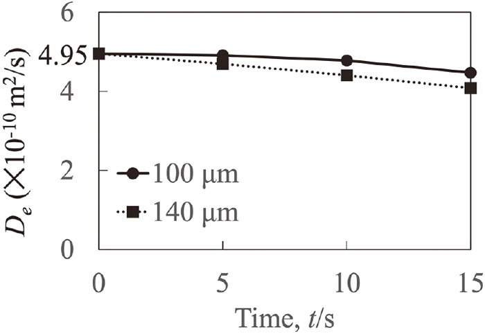
Fig. 4. Effective diffusion coefficient evaluation results under DC+MF condition.
Figure 5 indicates the effective diffusion coefficient evaluation results under the 2 Hz condition. The effective diffusion coefficients at the two evaluation positions were much smaller than 4.95×10⁻¹⁰ m2/s at 5 s, and these values decreased with time. Because the effective diffusion coefficient difference in each 5 s time interval was much larger than that caused by diffusion, the effect of convection on the time-variation of the effective diffusion coefficient might be dominant. The evaluated effective diffusion coefficients between at 100 μm and 140 μm were very close and their difference was less than 1.5×10⁻¹¹ m2/s. Notably, the effective diffusion coefficients under the 2 Hz condition were much smaller than that under the DC+MF condition. This means that the flow might be enhanced under the 2 Hz condition compared to that under the DC+MF condition.

Fig. 5. Effective diffusion coefficient evaluation results under 2 Hz condition.
Figure 6 indicates the effective diffusion coefficient evaluation results under the 6 Hz condition. The effective diffusion coefficients at the two measurement positions decreased with time. Similar to those under the DC+MF and the 2 Hz conditions, the flow excitation might be the main reason for the time decrease of the effective diffusion coefficient. In addition, the effective diffusion coefficients at 140 μm were smaller than those at 100 μm, and their difference increased with time. These mean that the flow might develop with time, and its velocity at 140 μm might be larger than that at 100 μm. Because the effective diffusion coefficients under the 6 Hz and the 2 Hz conditions were smaller than those under the DC+MF condition, the flow might be enhanced by imposing the time-varying electromagnetic force compared to that under the imposition of the static electromagnetic force. Furthermore, the effective diffusion coefficients under the 6 Hz condition were larger than that under the 2 Hz condition.

Fig. 6. Effective diffusion coefficient evaluation results under 6 Hz condition.
Figure 7(a) shows the liquid flow pattern near the anode surface under the DC+MF condition. Because the magnetic field intensity near the anode surface of 0.267 T was larger than that near the cathode surface of 0.264 T, a circulating macro-scale flow was excited in the whole vessel, and its flow pattern in the whole vessel was essentially the same with that in the previous study.18) The direction of the circulating macro-scale flow was the positive x-direction in the observation range.
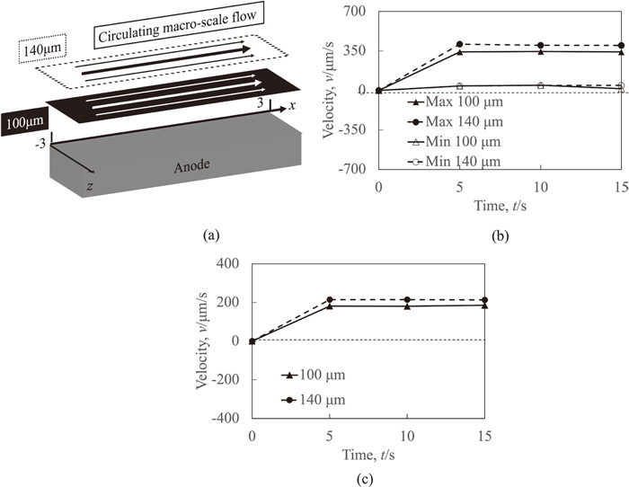
Fig. 7. (a) Liquid flow pattern from 5 s to 15 s, (b) maximum velocity and minimum velocity measurement results and (c) average velocity calculation results under DC+MF condition.
Figures 7(b) and 7(c) show the maximum and the minimum velocity measurement results and the average velocity measurement results under the DC+MF condition, respectively. A large velocity difference between the maximum velocity and the minimum velocity was observed, as shown in Fig. 7(b). Notably, the minimum velocity was very close to 0 at the two measurement positions. This was because the velocity at the side walls in the z-direction must be 0. The maximum velocity and the average velocity at 100 μm with magnitudes of about 340 μm/s and 180 μm/s were smaller than those at 140 μm with magnitudes of about 400 μm/s and 210 μm/s, respectively, because the latter was far from the anode surface. Because of the flow excitation, the liquid with the initial Cu2+ concentration flowed from the bulk region to the adjacent region of the anode surface. This suppressed the Cu2+ concentration increase near the anode surface. Thus, the flow development suppressed the concentration boundary layer development. This was the reason why the effective diffusion coefficient decreased and the mass transfer enhanced with the flow development. Therefore, the effective diffusion coefficients decreased with time and the effective diffusion coefficient at 140 μm was smaller than that at 100 μm, as shown in Fig. 4.
Figure 8(a) shows the liquid flow pattern observation results near the anode surface under the 2 Hz condition. Particle motions in both the positive and the negative x-directions were simultaneously observed near the middle part of the anode surface at the y-positions of 100 μm and 140 μm. This means a circulating micro-scale flow was excited, and the liquid flow pattern under the 2 Hz condition was different from that under the DC+MF condition.

Fig. 8. (a) Liquid flow pattern from 5 s to 15 s, (b) maximum velocity and minimum velocity measurement results and (c) average velocity calculation results under 2 Hz condition.
Figures 8 (b) and 8(c) show the velocity measurement results at 100 μm and at 140 μm under the 2 Hz condition. Because the circulating micro-scale flow included the negative x-direction velocity component, the minimum velocity was the negative value. The average velocities of particles moving in the positive x-direction and the negative x-direction were calculated separately. These average velocities were named as the ‘positive average velocity’ and the ‘negative average velocity’, respectively. The maximum velocity at 100 μm was very close to that at 140 μm, and the positive average velocity, the absolute values of the minimum velocity and the negative average velocity showed similar tendency. The magnitudes of the maximum velocity and the absolute value of the minimum velocity were essentially the same, as shown in Fig. 8(b). These values slightly increased from about 500 μm/s at 5 s to about 600 μm/s at 15 s. Similar tendency was also observed in the average velocity calculation results, as shown in Fig. 8(c). The positive average velocity and the absolute value of the negative average velocity increased from about 270 μm/s at 5 s to about 360 μm/s at 15 s. These are the reasons that the effective diffusion coefficients were very close between at 100 μm and 140 μm, and these values decreased with time as shown in Fig. 5.
Figures 9(a) and 9(b) show the observed liquid motion near the anode surface under the 6 Hz condition. The liquid flow pattern changed with time. Only the circulating macro-scale flow was observed at the two observation positions at 5 s and 10 s, as shown in Fig. 9(a). At 15 s, both the circulating macro-scale flow and the circulating micro-scale flow were observed at 140 μm, whereas only the circulating macro-scale flow was observed at 100 μm, as shown in Fig. 9(b). Compared to that under the 2 Hz condition, the time for exciting the circulating micro-scale flow increased. This means that the excitation of the circulating micro-scale flow might depend on the frequency of the time-varying electromagnetic force. However, the mechanism of the circulating micro-scale flow excitation by imposing the time-varying electromagnetic force has not been clarified at this stage, and this will be further investigated in future work.

Fig. 9. (a) Liquid flow pattern from 5 s to 10 s, (b) liquid flow pattern from 10 s to 15 s, (c) maximum velocity and minimum velocity measurement results and (d) average velocity calculation results under 6 Hz condition.
The velocity evaluation results under the 6 Hz condition were shown in Figs. 9(c) and 9(d). Similar to that under the DC+MF condition, the magnitudes of the minimum velocity at the two measurement positions were close to 0 at 5 s and 10 s. At 15 s, the minimum velocity slightly increased at 100 μm because of the development of the circulating macro-scale flow. And that value at 140 μm was −350 μm/s because of the excitation of the circulating micro-scale flow. The negative average velocity was 0 at 100 μm from 5 s to 15 s and at 140 μm from 5 s to 10 s because of the same reason. The excitation of the circulating micro-scale flow was considered as one of the reasons of the lower effective diffusion coefficient at 140 μm, as shown in Fig. 6. On the other hand, the maximum and positive average velocities at 140 μm was larger than that at 100 μm. This was another reason for the lower effective diffusion coefficient at 140 μm. The maximum velocities at 5 s were almost the same with that at 10 s. Their magnitudes were 360 μm/s and 450 μm/s at 100 μm and 140 μm, respectively. At 15 s, the maximum velocity increased to the magnitudes of 480 μm/s and 530 μm/s at 100 μm and 140 μm, respectively. In addition, the magnitudes of positive average velocities at 5 s and at 10 s were 190 μm/s and 250 μm/s at 100 μm and at 140 μm, respectively. And their value increased to around 300 μm/s and 320 μm/s at 100 μm and at 140 μm, respectively.
Figure 10 shows the maximum velocity measurement results and the effective diffusion coefficient evaluation results under the experimental conditions with the superimposition of the current and the magnetic field. The magnitudes of the maximum velocities at 100 μm and 140 μm under the 2 Hz condition and the 6 Hz condition were larger than those under the DC+MF condition, as shown in Figs. 10(a) and 10(b). Similar results were also observed in the positive average velocity calculation results, as shown in Figs. 7(c), 8(c) and 9(d). Therefore, the flow was enhanced under the former two conditions compared to that under the DC+MF condition. Because the mass transfer enhanced and the effective diffusion coefficient decreased with the flow development, the mass transfer under the 2 Hz condition and the 6 Hz condition was enhanced compared to that under the DC+MF condition, and the effective diffusion coefficients under the former two conditions were smaller than those under the DC+MF condition, as shown in Figs. 10(c) and 10(d). In addition, the magnitudes of the maximum velocities under the 2 Hz condition were larger than those under the 6 Hz condition, as shown in Figs. 10(a) and 10(b). Therefore, the effective diffusion coefficients under the 2 Hz condition were smaller than those under the 6 Hz condition, and the mass transfer under the 2 Hz condition was enhanced compared to that under the 6 Hz condition.

Fig. 10. Maximum velocity measurement results under experimental conditions with current and magnetic field superimposition at (a) 100 μm and (b) 140 μm, and effective diffusion coefficient evaluation results at (c) 100 μm and (d) 140 μm.
4. Conclusion
To investigate the effects of the time-varying electromagnetic force and its frequency on mass transfer near the solid-liquid interface, the effective diffusion coefficient, which reflects the effect of the flow on the time variation of the solute concentration, was evaluated just above the solid-liquid interface. The following results were obtained:
(1) By imposing the electromagnetic force, the effective diffusion coefficient was smaller than the diffusion coefficient because of the flow excitation.
(2) By imposing the time-varying electromagnetic force, the effective diffusion coefficient was decreased compared to that under the imposition of the static electromagnetic force, though the average force intensities were the same. This meant that the mass transfer was enhanced by imposing the time-varying electromagnetic force. This was because the flow was enhanced by imposing the time-varying electromagnetic force.
(3) The effective diffusion coefficient under the 2 Hz condition was smaller than that under the 6 Hz condition. This meant that the mass transfer might be enhanced by decreasing the time-varying electromagnetic force frequency. This was because the flow was enhanced under the 2 Hz condition compared to that under the 6 Hz condition.
(4) The liquid flow pattern under the imposition of the time-varying electromagnetic force was different from that under the imposition of the static electromagnetic force.
(5) The time for the excitation of the circulating micro-scale flow under the 2 Hz condition was shorter than that under the 6 Hz condition. This meant that the excitation of the circulating micro-scale flow might depend on the frequency of the time-varying electromagnetic force.
References
- 1) K. Iwai, T. Yokota, A. Maruyama and T. Yamada: IOP Conf. Ser: Mater. Sci. Eng., 424 (2018), 012051. https://doi.org/10.1088/1757-899X/424/1/012051
- 2) D. Landolt: J. Electrochem. Soc., 149 (2002), S9. https://doi.org/10.1149/1.1469028
- 3) E. L. Cussler: Diffusion: Mass transfer in fluid systems, Cambridge university press, New York, (2009), 2.
- 4) J. D. Madden and I. W. Hunter: J. Microelectromech. Sys., 5 (1996), 24. https://doi.org/10.1109/84.485212
- 5) I. Manabu and J. I. Olusegun: Basic Transport Phenomena in Materials Engineering, Springer, Tokyo, (2014), 141.
- 6) R. B. Bird, W. E. Stewart and E. N. Lightfoot: Transport Phenomena, John Wiley & Sons, Inc., New York, (2007), 621.
- 7) T. Yokota, A. Maruyama and K. Iwai: Tetsu-to-Hagané, 102 (2016), 119 (in Japanese). https://doi.org/10.2355/tetsutohagane.TETSU-2015-095
- 8) E. K. Ramasetti, V. V. Visuri, P. Sulasalmi, T. Fabritius, T. Saatio, M. Li and L. Shao: Metals, 9 (2019), 829. https://doi.org/10.3390/met9080829
- 9) E. K, Ramasetti, V. V. Visuri, P. Sulasalmi, T. Fabritius, J. Savolainen, M. Li and L. Shao: Metals, 9 (2019), 1048. https://doi.org/10.3390/met9101048
- 10) T. M. Schobeiri: Fluid Mechanics for Engineers A Graduate Textbook, Springer, Berlin, (2010), 2.
- 11) V. L. Streeter: Fluid Mechanics, McGraw-Hill Book Company, INC., New York, (1958), 161.
- 12) L. G. Leal: Advanced Transport Phenomena: Fluid Mechanics and Convection Transport, Cambridge University Press, New York, (2007), 598.
- 13) M. Iguchi, J. Yoshida, T. Shimizu and Y. Mizuno: ISIJ Int., 40 (2000), 685. https://doi.org/10.2355/isijinternational.40.685
- 14) T. Yokota, A. Maruyama, T. Yamada and K. Iwai: J. Japan. Inst. Met. Mater., 81 (2017), 516 (in Japanese). https://doi.org/10.2320/jinstmet.J2017022
- 15) Y. Zhang, G. Ding, H. Wang and P. Cheng: J. Electrochem. Soc., 162 (2015), D427. https://doi.org/10.1149/2.0111509jes
- 16) E. Shvydkiy, E. Baake and D. Köppen: Metals, 10 (2020), 532. https://doi.org/10.3390/met10040532
- 17) W. Zhu, S. Yu, C. Chen, L. Shi, S. Xu, S. Shuai, T. Hu, H. Liao, J. Wang and Z. Ren: Metals, 11 (2021), 1846. https://doi.org/10.3390/met11111846
- 18) G. Xu and K. Iwai: ISIJ Int., 62 (2022), 1389. https://doi.org/10.2355/isijinternational.ISIJINT-2021-177
- 19) D. F. Swinehart: J. Chem. Educ, 39 (1962), 333. https://doi.org/10.1021/ed039p333
- 20) T. G. Mayerhöfer, H. Mutschke and J. Popp: Chem Phys Chem., 17 (2016), 1948. https://doi.org/10.1002/cphc.201600114
- 21) N. Kanani: Electroplating: Basic Principles, Processes and Practice, Elsevier, Kidlington, (2004), 116.
- 22) E. E. Stansbury and R. A. Buchanan: Fundamentals of Electrochemical Corrosion, ASM International, State of Ohio, (2000), 108.
- 23) K. Fueki: Denkikagakubenran, Maruzen, Tokyo, (1985), 158 (in Japanese).
- 24) D. Forster, D. R. Nelson and M. J. Stphen: Phys. Rev. A., 16 (1977), 732. https://doi.org/10.1103/PhysRevA.16.732
- 25) H. Kitahata and N. Yoshinaga: J. Chem. Phys., 148(2018), 134906. https://doi.org/10.1063/1.5021502
- 26) T. H. Solomon and J. P. Gollub: Phys. Fluids., 31 (1988), 1372. https://doi.org/10.1063/1.866729
- 27) A. Emanuel and D. R. Olander: J. Chem. Engng Data., 8 (1963), 31. https://doi.org/10.1021/je60016a008
- 28) W. G. Eversole and H. M. Kindsvater: J. Phys. Chem., 3 (1942), 370. https://doi.org/10.1021/j150417a006

