Original Paper
Oscillationless Explicit Method on Overset Grid for Advective Equation
2013 Volume 16 Pages 1-11
Details
2013 Volume 16 Pages 1-11
Characteristics of numerical errors using the overset grid method are investigated. The overset grid method has some problems with the interpolation of data between each mesh. In the case of the computing advective equation, a traveling wave passing through an interface of overlapping meshes causes numerical oscillations. The oscillations near the interface destroy the solution, and cause overflow. In order to investigate the causes of the numerical errors on the overset grid, we apply wave analysis on each component mesh. We show that phase differences between component meshes cause the numerical errors and that the accuracy of the phase velocity is quite important to compute the advective equation with less numerical errors on the overset grid. We suggest that calculations using accurate phase velocity will reduce numerical errors. We show that CIP scheme is one of the most useful schemes to represent wave propagation with high accuracy and without oscillation on the overset grid.
An overset grid method (Benek et al., 1983; Steger et al., 1983; Benek et al., 1985), which is sometimes called a chimera grid method, provides a flexible and efficient spatial discretization procedure to solve a wide variety of complex problems (Belk, 1995; Burton and Eaton, 2002; Carlsson and Petersson, 2001; Dwyer, 1994; Henshaw, 1994; Kageyama and Sato, 2004). The overset grid is composed of the several meshes which cover the whole computational domain. Each mesh of the overset grid is independently generated as simply as orthogonal rectilinear mesh. Therefore the overset grid method offers relative advantages of cost for generating meshes compared with unstructured grids. Moreover, since the calculation schemes are used independently in each mesh, we can use differential or interpolation schemes for simple mesh such as orthogonal rectilinear mesh. It does not require us to develop particularly complicated schemes for the overset meshes.
However, the overset grid method has problems with interpolation in the overlapping regions. CFD simulation using the overset grid method frequently generates numerical oscillations near the interface of each component mesh. Such oscillations may destroy the solution and cause overflow.
Generally, computational costs in the explicit integration scheme are much less than in the implicit integration scheme. But the completely stable and non-oscillatory method for the explicit integration scheme does not exist as Starius (1977, 1980) proved, although a number of methods to suppress numerical oscillation have been proposed by many authors (Berger, 1987; Moon and Liou, 1989; Pärt-Enander and Sjögreen, 1994; Fujii, 1995; Wang, 1995, 2001).
In this paper, we focus on numerical errors on overset grids with the explicit integration scheme for advective equations. In order to investigate the causes of the oscillatory behavior at the interface, we apply wave analysis for waves passing through each component mesh. We also propose method to suppress numerical errors on the overset grid.
This paper is composed as follows. After the introduction, the configurations of the overset grid method, which are mesh configurations and data exchange methods, are defined in section 2. In section 3, numerical simulations for two-dimensional advective equation are implemented. Wave analysis is applied for waves on each component mesh in section 4. In section 5, we propose the way to suppress numerical oscillations at the interfaces of the overlapping meshes. The conclusions of this study are presented in section 6.
In the overset grid method, the number of component grids is not limited, but a two-grid system is sufficient to investigate numerical errors. An overset grid composed of three or more component meshes is a simple extension of the algorithm derived here.
The overset grid is characterized by a region of overlap which is locally defined by the following three properties.
We consider the computational domain of the two grid systems as Fig. 1. One component mesh is termed Ω1, which covers the whole computational domain (Fig. 1(a)). The other component mesh is termed Ω2, which rotates counterclockwise by angle α to Ω1 (Fig. 1(b)). The side lengths, the number of grids per side and the boundary of the mesh are termed L1, N1, ∂Ω1 in Ω1, and L2, N2, ∂Ω2 in Ω2, respectively. It is important to note that Ω1 has a non-computational area at the center of its mesh, Ω0, which is whole covered by Ω2 (Fig. 1(c)). The overlapping area between Ω1 and Ω2 is the gray area in Fig. 1(c). In Fig.1, the circles and squares denote the grid points inside the meshes and the grid points on the boundary of the meshes, respectively. The white and black colors of the marks (circles and squares) are related to Ω1 and Ω2, respectively.

The computational domain using the overset grid method. Solid and dashed lines correspond to Ω1 and Ω2, respectively. The Ω1 and the Ω2 are overlapped with angle α. The overlapping region is represented as gray region, and the circles and squares denote the grid points inside the meshes and the grid points on the boundary of the meshes, respectively.
We examine two types of data exchange methods between two meshes. In one method, we define the boundary values of one mesh by interpolating the data from the other mesh. This method is called boundary exchange method (BEM) which is commonly used on overset grids (Starius, 1977, 1980; Pärt-Enander and Sjögreen, 1994; Burton and Eaton, 2002). The other method is called regional exchange method (REM). In this method, we exchange the data over the overlapping region.
The detail of BEM from Ω2 to Ω1 is as follows. We exchange the values of the grid points only on the boundary of the overlapping region, and the values of the grid points except the boundary are calculated by an equation for each mesh. The values on ∂Ω1 are obtained by interpolation from neighboring grid points on Ω2. The values on ∂Ω2 are obtained the same as Ω1. Because the information is exchanged only on the boundary of each mesh, the information of the grid points except for the boundary are not exchanged even though we calculate the same overlapping region for each mesh.
On the other hand, the detail of REM from Ω2 to Ω1 is as follows. A value from the overlapping region is obtained as the mean value between the value obtained from the governing equation and the interpolated value of the other mesh. The value on the boundary lines of the overlapping region for REM is defined the same as for BEM. Whereas the interpolated points of BEM are around the line of the boundaries, which of REM is on the face of the overlapping regions. The number of grid points on the overlapping regions is more than the number of grid points on the boundary lines of the overlapping regions. Therefore, since the number of grid points in which the data is exchanged is greater in REM than in BEM, the computational cost of REM is higher than BEM.
In order to investigate the causes of the numerical errors on the overset grid, we calculate the 2-dimensional advective equation using some cases of the parameters (i) ratio of grid size γ = (L2/N2) / (L1/N1) and (ii) angle between two meshes α. The normalized 2-dimensional advective equation is as follows.
 | (1) |
where h and  are a normalized scalar variable and advective velocity, respectively. Initial condition of the scalar variable h has a periodic wave configuration as follows.
 | (2) |
where k is a wavenumber k = 2mπ/L1, in which m (= 1, 2, 3, … ) is the number of the waves in the computational domain. The vector  is an x-directional stationary flow:
  = (1, 0).
We set the conditions for the experiments as follows. The L1, L2 and N1 are equal to 1, 1/2 and 80, respectively. We consider three cases of N2; 40, 30 and 80. Under these conditions, the ratios of grid sizes between the meshes γ are 1, 4/3 and 1/2, respectively. In addition, we set the angle between two meshes α to 0 and π/4.
We discretize the equation (1) using 2nd order central differential scheme (CDS) for space derivative, and 4th order Runge-Kutta scheme for the time integral. Fifth order Lagrange interpolation scheme is used for the data exchange method. The CFL number for the smallest grid size is 0.8 for the experiments in all cases in order to guarantee stable time integration throughout the experiments. The number of waves over the computational domain m is set to be 8. Because the wavenumber k becomes 16π/L1 = 2π/(10Δx1), one wave is represented using ten grid points.
3.2. Simulation resultsThe simulation results of advective experiments at τ = 1.0, where τ is normalized time, are shown in Fig. 2, Fig. 3, Fig. 4 and Fig. 5. Fig. 2 shows 2-dimensional scalar value distribution using BEM. The variable h on Ω2 is shown by the inner solid square region, and the value on Ω1 is shown in the outer regions of these figures. The dashed square corresponds to Ω0.

The value of scalar variable h using BEM at τ =1.0. Upper and lower figures are the results on α = 0 and π/4, respectively. The resolutions (or grid numbers) of figures are (a)(d) N2= 40, (b)(e) N2= 30 and (c)(f) N2= 80, respectively.

The spectral intensity using BEM at τ =1.0. The horizontal axis represents a number of waves m. Upper and lower figures are the results on α = 0 and π/4, respectively. The resolutions (or grid numbers) of figures are (a)(d) N2= 40, (b)(e) N2= 30 and (c)(f) N2= 80, respectively.

Simulation results using REM at τ = 1.0.

The spectral intensity using REM at τ = 1.0.
In Fig. 2(a), (b) and (c), the angles between Ω1 and Ω2 are zero (α = 0), and the grid numbers N2 are 40, 30 and 80, respectively. The simulation result of N2= 40 and α = 0 (Fig. 2(a)) is the same as that of one rectilinear mesh, because the grid size of Ω2 is the same as that of Ω1 and there is no angle between the two meshes. In Fig. 2(b) and (c), which are the results of N2= 30 and N2= 80, numerical oscillations occur around the interface of the overlapping meshes. Therefore it turns out that the numerical errors are generated by the difference of resolution between the two meshes.
The results of α = π/4 are shown in Fig. 2(d), (e) and (f). Comparing Fig. 2(a) and (d), numerical oscillations are induced by inconsistencies of the grid angles α. On the other hand, using the coarse resolution N2= 30, the numerical oscillations are small.
We plot the spectral intensity in x-direction for BEM in Fig. 3. The horizontal axis in these figures represents the number of waves (m = kL1/2π). The diffused profiles from reference wave form (Fig. 3(a)) indicates the numerical errors over the advective calculations in Fig. 3(b)–(f). In addition, the numerical oscillations of N2= 30 and α = π/4 were smaller than that of other conditions.
Simulation results using REM are shown in Fig. 4 and Fig. 5 Waves in Fig. 4 are warped out of shape in some cases. The top of the wave in N2= 30 and α = 0 is delayed compared with N2= 40, and the top of the wave in N2= 80 is advanced. In the result of α = π/4, the waves in N2= 40 and N2= 80 are advanced, while the waves of N2= 30 are almost unaffected. Comparing Fig. 3 and Fig. 5, the numerical oscillations in REM become smaller than in BEM.
In this section, we discuss the wave analysis in Ω2. Here we think about x′–y′ coordinates which are rotated from x–y coordinates with the angle of α. The x–y and x′–y′ coordinates are parallel with Ω1 and Ω2, respectively (Fig. 1). When the advective direction is set to x-direction, the velocity in x′–y′ coordinate becomes  = (cosα,−sinα). If we assume that the wave solution is h = h0 exp[i(ωt−kx′x′−ky′y′)], the discrete advective equation in x′–y′ coordinate becomes the following form.
 | (3) |
where δx′ , δy′ and f(x) are defined as follows.
 | (4) |
 | (5) |
 | (6) |
Assuming the time step is sufficiently small, we can analytically calculate the time derivative [∂h/∂t]i,j = iωhi,j. Then the phase velocity vp = ω/k becomes
 | (7) |
 | (8) |
 .
.
The relation between the phase velocity vp and the wavenumber k for the case of Δy′ = Δx′ is shown in Fig. 6. The lines A1 and A2 correspond to the phase velocities when γ = 1. Similarly, the lines B1 and B2 are used when γ = 4/3, and the lines C1 and C2 are used when γ = 1/2.

The discrete phase velocity using 2nd order CDS. Solid line denotes the phase velocity on α = 0, and dashed line denotes the phase velocity on α =π/4. Circle (◯) and triangle (Δ) and cross (×) on the lines correspond to γ = 1, 4/3 and 1/2, respectively.
When N1 = 80, which is same condition of previous section, the phase velocity of γ = 1, 4/3 and 1/2 correspond to the phase velocities in Ω2 for the cases when N2= 40, 30 and 80, respectively. Therefore, the phase velocities A1 , B1 and C1 represent the phase velocities in Ω2 for the cases of N2= 40, 30 and 80 on α = 0, and the lines A2 , B2 and C2 represent the phase velocities for the cases of N2 = 40, 30 and 80 on α = π/4, respectively. Since the phase velocity in Ω1 is the same as that in the case of N2 = 40 and α = 0, the line A1 corresponds to the phase velocity in Ω1.
The wavenumber of the above experiments shown in Fig. 2 and Fig. 4 is k = 2π/(L1/8) = π/5Δx. The phase velocity of this wavenumber is shown in Table 1. The phase velocity of B2 is largely similar to that of A1. Since the differences of the phase velocities are very small, there are small numerical errors in Fig. 2(e) and Fig. 4(e). On the other hand, since other cases have large differences of phase velocity, the phase differences between the meshes are amplified during the calculation. In the case of BEM, since data are exchanged only at the boundary lines of the overlapping regions, phase differences cause data differences at the boundary of the overlapping region, and small wavelength waves are generated from the boundary lines. In cases of REM, the phase differences disappear by the averaging operation over the overlapping region. However, the waves are varied in the phase and are warped out of wave shape.
| A1 | B1 | C1 | A2 | B2 | C2 | |
|---|---|---|---|---|---|---|
| vp | 0.936 | 0.887 | 0.984 | 0.967 | 0.944 | 0.992 |
| ratio | 100.00% | 94.82% | 105.18% | 103.41% | 100.75% | 106.02% |
The numerical errors in Fig. 2 and Fig. 4 would come from the errors related to the discrete dispersion relation characterized by parameters γ and α. The phase velocity vp, which is written in equation (8), monotonically increases as γ or cos α increase (α ∈ [0, π/4]). Therefore the phase velocity becomes larger as the ratio of grid sizes increases or as the x′−y′ coordinates rotate from the x−y coordinates. If the dispersion relation is different between component meshes, the phase velocities in the overlapping regions are not the same. The difference of the phase velocity causes the phase difference and numerical errors in the overlapping region.
On the other hand, the phase difference is also proportional to the difference in the time while one wave moves over the overlapping region. Therefore, the small size of the overlapping region reduces the phase difference. However, the numerical error is not proportional to the phase difference between the meshes, except when the phase difference is smaller than a half the wave length. In most of the simulation of the nonlinear problem, the size of the overlapping region needs to be sufficiently smaller than the grid size in order to suppress the numerical errors in any scale of waves, since many scales of phase differences occur in these systems. However, it is not realistic that the width of the overlapping region is smaller than the grid size in whole overlapping region.
As discussed previously, there are numerical errors in the overset grid method such as oscillations for BEM and deformation of waves for REM. In order to avoid such numerical errors, it is effective to reduce the phase differences between the meshes. Namely, the numerical errors are suppressed if the discrete wave dispersion relation is independent of the grid size and the advective direction.
One method is to use such a higher order differential scheme. The phase velocities using 2nd, 4th, 6th and 8th order CDS are shown in Fig. 7. The phase velocity becomes more accurate when using the higher order scheme.

Phase velocity vp for 2nd, 4th, 6th and 8th order CDS and CIP scheme on α = 0. Because the phase velocity for CIP scheme depends on CFL number, we use some kind of CFL number; 0.2, 0.5 and 0.8.
We calculate the wave advective equation with the same condition as section 3 (advective simulation) using 8th order CDS. The mesh condition is N2= 80 and α = π/4. This was the condition when the numerical errors were the largest in previous simulation results using 2nd order CDS.
Fig. 8(a), (b) are simulation results using BEM and REM, respectively, and Fig. 9(a), (b) show spectral intensity in x-directional of Fig. 8(a), (b), respectively. The numerical errors in these figures are very small. In both cases, BEM and REM, the difference of phase velocities between the meshes is 3 × 10⁻⁵. Therefore, this scheme reduces the phase difference between the meshes.

Simulation results for m = 8 using 8th order CDS. The condition of the Ω2 is α = π/4 and N2= 80 (γ = 1/2).

Simulation results for m = 8 using 8th order CDS. The condition of the Ω2 is α = π/4 and N2= 80 (γ = 1/2).
However, calculations of smaller wavelength mode (namely, larger number of waves) have different results. Simulation results for m = 20 (k = π/2Δx′) using the 8th order CDS are shown in Fig. 10, and spectral intensity of these results are shown in Fig. 11. The numerical oscillation similar to that of Fig. 2(f) appears in the result using BEM in Fig. 10(a). On the other hand, in the result using REM in Fig. 10(b), the wave becomes smaller in amplitude and gradually disappears. Since the phase velocities in Ω1 and Ω2 for this case are 0.970 and 1.000 respectively, there is about 3% difference in phase velocity. Therefore, the phase difference increases in the overlapping region, and the numerical oscillation or the amplitude decay occurs as shown in Fig. 10. In order to suppress numerical errors in the smaller wavelength mode, we should use the higher order scheme.

Simulation results for m = 20 using 8th order CDS. The condition of the Ω2 is α = π/4 and N2= 80 (γ = 1/2).
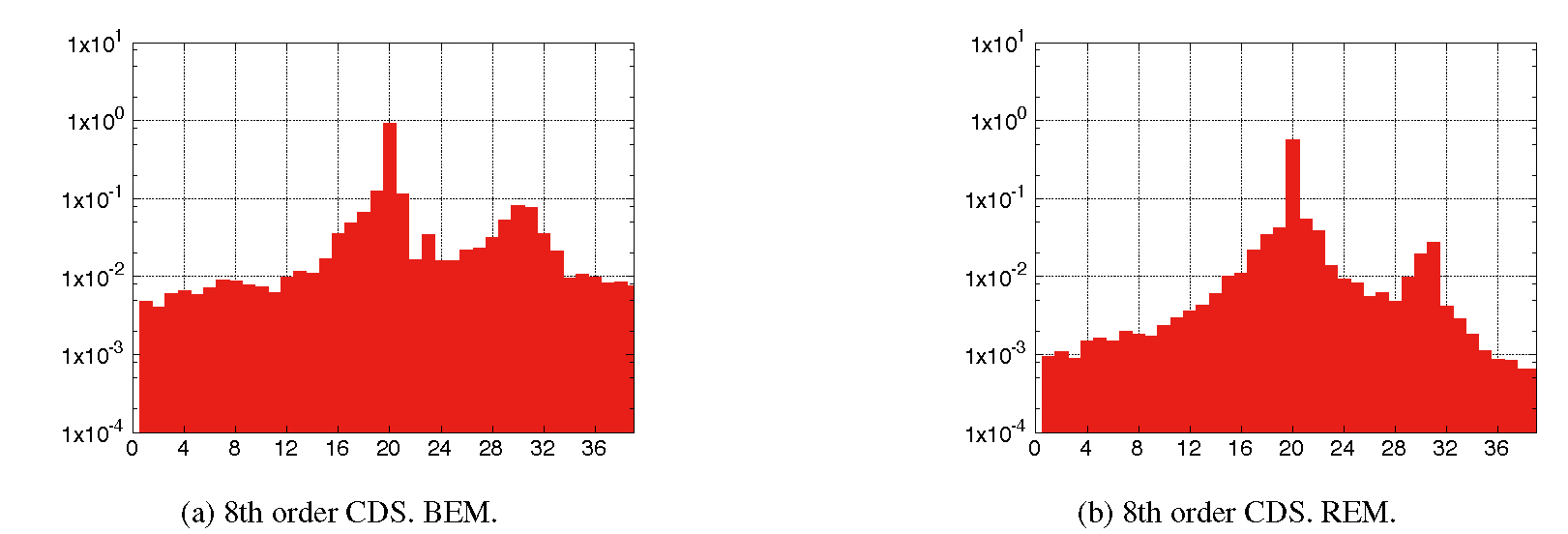
Spectral intensity of the simulation results for m = 20 using 8th order CDS. The condition of the Ω2 is α = π/4 and N2= 80 (γ = 1/2).
Multi-Moment scheme (Yabe and Aoki, 1991) is another type of higher order scheme. In this scheme, we use not only the point variables but also other type of variables (e.g. integral variables, derivative variables) in order to construct a higher order interpolation. CIP scheme (Yabe et al., 2005), which is a Multi-Moment scheme, can represent the correct phase velocity for advective equations. Phase velocity using the CIP scheme is shown in Fig. 7 (Utsumi et al., 1997). From Fig. 7, we can see that the CIP scheme gives the correct phase velocity with very small numerical dispersion not only for small wavenumber components but for large wavenumber components. In this section, we calculate wave advection using the same condition as section 5.1 using B-type CIP scheme (Aoki, 1995).
Simulation results in Fig. 12, when m = 8, show few numerical oscillation and a little deformation of waves. The results are due to the correct phase velocity given by the use of CIP scheme. This calculation result is similar to 8th order CDS in Fig. 8.

Simulation results of advective equation using CIP scheme. The number of waves is m = 8. The figures (a)(b) are 2-dimensional configuration and figures (c)(d) are spectral intensity. The data exchange method is (a)(c) BEM and (b)(d) REM, respectively. The condition of the Ω2 is N2= 80 and α = π/4.
The CIP scheme also shows small numerical errors with m = 20 (Fig. 13) because the phase velocity has very small dispersion errors as shown in Fig. 7. This behavior in the short wavelength indicates clear advantage of CIP method over 8th order CDS.

Simulation results of advective equation using CIP scheme. The number of waves is m = 20. The figures (a)(b) are 2-dimensional configuration and figures (c)(d) are spectral intensity. The data exchange method is (a)(c) BEM and (b)(d) REM, respectively. The condition the of Ω2 is N2= 80 and α = π/4.
By these results, CIP scheme offers advantages in suppression of numerical errors for a wide range of wavelength components compared with CDS scheme. Although we use B-type CIP scheme for advective simulation in this paper, we can also obtain similar results using other schemes to represent correct phase velocity, for example conservative CIP scheme (Tanaka et al., 2000; Yabe et al., 2001) or rational function CIP scheme (Xiao et al., 1996).
Numerical errors in the overset grids were investigated by calculating wave advection and applying wave analysis. We found that phase differences between component meshes cause numerical errors in the overset grid. The phase differences in the overlapping regions came from differences of the phase velocity characterized by grid size and differential scheme. We showed that no differences in the phase velocity between component meshes are effective suppressing the numerical errors. This was accomplished by using high accuracy schemes to represent correct phase velocity.
Calculation using CIP scheme can represent the phase velocity with high accuracy for advective equations. Different from the high order CDS, the discrete dispersion error using CIP scheme was almost independent of wavenumber. Therefore, we can suppress the numerical errors in the overset grids by using CIP scheme for advective equations. By these results, it is effective in the overset grids to use the differential scheme with high accuracy in phase velocity, as well as just the high order differential scheme.
In most simulations of nonlinear problems, many scales of waves appear and mutually interact. For example, a gravity wave at atmosphere with a small scale of time and space carries energy and momentum, and emits the energy when the wave breaks up. This phenomenon has wide impacts for the large scale phenomena such as the global thermal balance and the jet stream in the troposphere. Therefore, we would like to use high accuracy scheme which can represent the phenomena of wide range of wavelength components. In calculations with fixed resolution using differential scheme, small wavelength mode characterized by grid size necessarily appear. Since numerical errors in the overset grid method are caused by small wavelength components in the overlapping regions, it is necessary to use differential scheme with high accuracy in the phase velocity in order to suppress the numerical errors.
I am grateful to members of Multiscale Simulation Research Group for providing helpful comments and suggestions. I would also like to express my gratitude to my family for their moral support and warm encouragements.